Information in these Priority Topics was prepared to supplement the information for Physical and Chemical Properties published in Section 4, Fate and Transport published in Section 5, Site Characterization published in Section 10, and Surface Water Quality in Section 16. Information about Strategic Environmental Research and Development Program (SERDP) and Environmental Security Technology Certification Program (ESTCP) projects for these topics can be found at https://serdp-estcp.mil/.
1.3.1 Vadose Zone Characterization and Transport
This section provides additional details on air-water partitioning behavior of PFAS and advances in vadose zone fate-and-transport modeling for PFAS. This content complements information in Section 4, Section 5, and Section 10. More specific references are provided for each subtopic.
1.3.1.1 Air-water Partitioning
Section 4.2.8, Section 5.2.4.1, and Section 5.3.3 describe how competing hydrophobic and hydrophilic properties characteristic of surfactants, and specifically PFAS, result in complex transport dynamics. The presence of PFAS in porewater lowers interfacial tension and forms films at the air-water interface (AWI), with the hydrophobic carbon-fluorine tail oriented toward the air and the hydrophilic head group dissolved in water. AWI partitioning can retard PFAS migration and reduce leaching potential, with site-specific factors such as soil texture, salinity, and pH influencing the extent of retention. AWI can vary spatially in response to soil texture and heterogeneities, and temporally in response to saturation and recharge events. This behavior can significantly affect PFAS transport in the vadose zone (Figure 1-1).
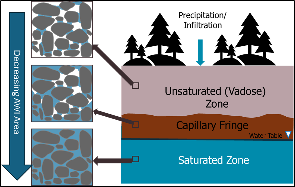
Figure 1-1. Partitioning and interfacial area. The degree of water saturation affects the amount of interfacial area in a nonlinear manner. Increased interfacial area increases retention. Factors that contribute to retention at the AWI include porewater ionic strength, PFAS concentration, and soil properties such as grain size, minerology, and moisture content, which affect the thickness of the capillary fringe.
Studies have shown that adsorption of PFAS such as perfluorooctane sulfonic acid (PFOS) and perfluorooctanoic acid (PFOA) at the AWI can retard transport, contributing to around 50% of total retention under certain test conditions, depending on site-specific parameters (Brusseau 2018; Bigler et al. 2024). This adsorption to the AWI can be assumed to be instantaneous (Guo et al. 2022). This section primarily summarizes recent research on this rapidly evolving topic, emphasizing the need for continued investigation and incorporation of AWI processes, in addition to vadose zone retention, into conceptual site models (CSMs) and, as the science advances, risk assessments.
Interrelated to vadose zone retention, AWI within the capillary fringe may also impact retention. Wallis et al. (2022) noted that prolonged periods of evapotranspiration exceeding rainfall result in periods of upward flux of PFAS mass, leading to evapoconcentration and associated persistence in the vadose zone. This process acts counter to downward flux to groundwater, as typically conceived. The capillary forces discussed above demonstrate the dynamic nature of the AWI and highlight factors to consider when evaluating PFAS retention in the vadose zone and capillary fringe.
The AWI area is influenced by both soil grain size and soil saturation. In particular, the AWI-saturation relationship is nonlinear, with high AWI at low saturation and zero AWI at full saturation (Guo, Zeng, and Brusseau 2020). For example, soils with higher percentages of silt and clay size particles typically support larger AWI areas than coarser grain soils for a given water saturation (Brusseau 2023). Brusseau noted that spatial variability in soil texture and soil moisture should be considered when evaluating AWI area. Similarly, temporal changes in soil saturation (from infiltration and drainage) also affect the AWI area and may be important to consider depending on the specific goals/objectives of the investigation. Specifically, Guo et al. (2022) showed that modeled long-term leaching of PFAS was adequately assessed assuming steady-state conditions. But modeling focused on short-term impacts of infiltration on AWI area and PFAS leaching should consider the dynamic nature of surfactant-induced flow, and rate-limited, nonlinear adsorption at solid-water and air-water interfaces. However, incorporating these factors comes with significant computational costs and the requirement for detailed input parameters. Last, it is noted that grain size also affects the extent of PFAS retention via conventional sorption methods, as discussed in Section 5.2.
Soil type (mineralogy, grain size, and surface area) and porewater ionic type and strength influence PFAS accumulation at the AWI. Coarser grain sizes having lower water content and more air-filled pore space can increase retention. The adsorption of PFAS at the AWI decreases with increasing concentration and increases with the number of perfluorinated carbons, indicating different retention behaviors for various PFAS (Silva, Martin, and McCray 2021). Additionally, Le et al. (2021) and Stults et al. (2023) both highlighted that increasing ionic strength significantly enhances PFAS accumulation and retention at the AWI. Le et al. (2021) demonstrated this effect through a mass-action model, showing orders-of-magnitude increases in adsorption with rising ionic strength. Stults et al. (2023) further emphasized the influence of ion type and concentration, refining predictive models by adding an empirical ionic strength correction factor accounting for these effects under environmentally relevant conditions. Both studies underscore the critical role of ionic strength in PFAS fate and transport. Note that tidally influenced sites could have significantly retarded PFAS transport due to a combination of higher ionic strengths in the vadose and saturated zones, as well as thickened capillary fringe. Understanding this retention behavior will support review of site-specific analytical results combined with soil profile data. Processes that contribute to retention of PFAS in the vadose zone are summarized in Figure 1-2. Refer to Section 1.3.8.6, and Table 1-7 for sampling and analysis recommendations for grain size, soil classification, moisture content, and cation/anion exchange capacity that relate to vadose zone partitioning and leaching.
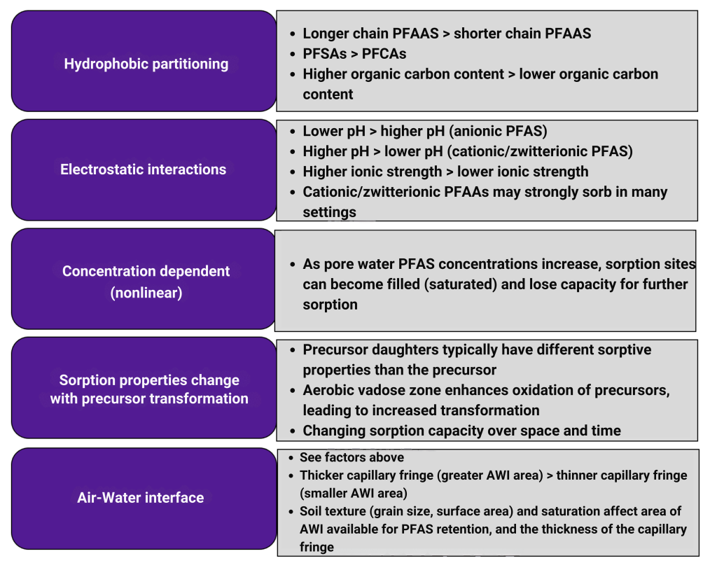
Figure 1-2. Factors influencing retention in the vadose zone.
Source: D. Drennan, BEM Systems. Used with permission.
Research has shown significant variability in leaching behavior across different soils, emphasizing the need for site-specific assessment. Thompson et al. (2024) highlighted the benefits of site-specific leaching tests for PFAS risk assessment, demonstrating variability in leaching among five different soils compared to modeled data based on regulatory assumptions. Navarro et al. (2024) described how laboratory-scale leaching tests provide controlled insights into PFAS behavior but struggled to replicate in situ conditions, particularly for the AWI. Laboratory leaching methods, including synthetic precipitation leaching procedure (SPLP) tests, often rely on simplified, saturated conditions over extended periods. This can overestimate the leaching from soils collected from the water table interface, as fully saturated conditions do not reflect the reality of the vadose zone, where saturation is transient and varies in both persistence and periodicity. Such methods overlook the important role of the AWI in PFAS accumulation and mobility, particularly for long-chain compounds. Ignoring adsorption to the AWI can result in soil screening levels that are significantly more stringent than otherwise (Brusseau and Guo 2023). As a result, standard tests may misrepresent leaching potential under field conditions. The observed variability in leaching behavior and the potential for laboratory studies to misrepresent leaching behavior together underscore the need for site-specific field validation approaches that account for climate, soil structure, wet-dry cycling, and variable saturation dynamics.
Recent microscale modeling by Chen and Guo (2023) provided additional insight into PFAS transport through the vadose zone. Their work showed that although PFAS can move efficiently within individual pores, its movement slows down significantly in areas where water is held tightly between grains and connectivity is limited. These restricted zones can delay PFAS release and cause extended periods of low-level contamination after initial breakthrough. This research reinforces the importance of accounting for small-scale retention processes when predicting PFAS movement through unsaturated soils.
Arshadi et al. (2024) compared 1-D simulations of aqueous film-forming foam (AFFF) -associated PFAS transport in the vadose zone to field observations. The study indicated that a large portion of the mass of PFOA and PFOS exists at the solid phase and the AWI. This tends to limit transport in the vadose zone. The rate of transport of PFAS in the aqueous phase is based on hydrogeologic properties, such as hydraulic conductivity and recharge rate. Their simulations also demonstrated the importance of considering the PFAS and other chemicals in the AFFF mixture because accumulation at interfaces is competitive and depends on the species present. Less surface–active PFAS (for example, shorter carbon chain length compounds such as perfluorohexane sulfonic acid (PFHxS), perfluorohexanoic acid (PFHxA), and perfluorobutane sulfonic acid (PFBS) (Guo, Saleem, and Brusseau 2023)) tend to have greater mobility when other chemicals are present.
Field studies also reveal gaps in our understanding of PFAS behavior at the AWI. Schaefer et al. (2024) used lysimeters to measure PFAS porewater concentrations at five AFFF-impacted sites, comparing field data with laboratory results from unsaturated soil cores and laboratory batch soil slurries. The study noted gaps in the scientific understanding of PFAS accumulation at the AWI. For instance, in the study PFAS accumulation at the AWI was orders of magnitude less than expected at two of the test sites. The research findings noted the potential importance of PFAS accumulation at the AWI in unsaturated soils and the impact of both soil texture and soil moisture content. The study also found that bench-scale testing of PFAS leaching and retention can be beneficial for understanding site-specific conditions but cautioned that improper accounting of AWI effects will result in misrepresentation of in situ leaching. The study noted significant concentrations of precursor compounds in 3 of 5 sites even after many years since original AFFF release. The authors stressed that sufficient understanding of precursor mass is essential for understanding long-term mass discharge and its role in the CSM. Last, the researchers noted that additional research is required to determine the extent to which their findings could be applied to more complex unsaturated zone conditions, such as dry and deep vadose zones with complex stratigraphy, and during extreme infiltration events. Disparities in field observations suggest a need to consider site-specific soil screening limits to account for wetting and drying cycles, soil texture, depth to water, and other parameters that may affect mass flux from the vadose zone. As such, vadose zone modeling techniques are being developed to define site-specific soil screening limits (Smith et al. 2024).
In a study of an AFFF-impacted site in a semi-arid region (27 cm average annual rainfall) where groundwater occurs at approximately 106 m below ground surface, researchers concluded that “99% of PFAS mass resided in the upper 3 m of the vadose zone” (Bigler et al. 2024). The researchers also noted that longer chain PFAS tended to remain within the uppermost (0–20 cm) portion of the vadose zone, while shorter chain PFAS accumulated at around approximately 1 m in depth, which is the top of a calcic horizon typically found in arid and semi-arid regions. PFAS of intermediate chain length were detected across the profile from surface to the calcic horizon (Bigler et al. 2024). It should also be noted that elevated PFAS concentrations (up to 40 ug/L) were observed along a 1- to 2-mile plume in deeper groundwater (water table at 100 m below land surface) in another portion of the site (USACE 2025), suggesting the importance of understanding subsurface heterogeneities that can affect PFAS in space and time.
1.3.1.2 Vadose Zone Modeling
Researchers from the University of Arizona have developed a comprehensive framework to model PFAS transport through the vadose zone (Brusseau and Guo 2023). Their research incorporated PFAS-specific retention mechanisms into the US Environmental Protection Agency’s (EPA’s) recommended process for determining migration to groundwater for soil screening levels (USEPA 1996); importantly, incorporation of these mechanisms can result in less stringent limits. Recently the Air Force Civil Engineer Center for Evaluation of Soil to Groundwater Leaching (AFCEC 2025) accepted this revised approach to developing the dilution attenuation factor. This does not necessarily imply regulatory acceptance, and practitioners should consult their specific regulators for guidance on how to determine a dilution attenuation factor and note that USEPA prefers multiple lines of evidence to support development of a site-specific dilution attenuation factor. The Smith, Brusseau, and Guo (2024) integrated modeling framework combines vadose-zone transport and groundwater dilution approaches, demonstrating that incorporating AWI retention is essential to accurately characterize PFAS contamination risks, particularly for longer chain PFAS.
The role of the AWI in PFAS retention and leaching is important but complex. Zeng and Guo (2023) conducted systematic numerical simulations to test the hypothesis that subsurface heterogeneities, such as soil texture, accelerate the migration of PFAS in soils. Their evaluations predicted that longer chain PFAS would be strongly retained in shallow soils but could also migrate to deeper soils in response to subsurface heterogeneities, such that heterogeneity-generated preferential flow reduces the AWI area accessible to PFAS and may accelerate migration more for longer chain PFAS than for shorter chain PFAS. Overall, the study suggested that characterizing and representing soil heterogeneities is critical for determining the accessible AWI area and accurately quantifying PFAS migration. This finding aligns with Stults et al. (2024), who used laboratory column studies and the HYDRUS 1-D model to show that while equilibrium models could predict total mass leaching, they failed to accurately forecast effluent porewater concentrations. A novel two-site leaching model incorporating AWI partitioning and rate-limited desorption provided better predictions, particularly for long-chain PFAS such as PFOS and PFOA. The uncertainty in leaching rates is much higher for long-chain than short-chain PFAS. The short-chain PFAS exhibit less retention in the vadose zone and are more uniformly distributed with depth, in part because solid-phase adsorption and AWI retention are comparatively weak for short-chain PFAS. The differences in leaching between short- and long-chain PFAS imply that while short-chain PFAS mass discharge to groundwater will tend to occur relatively quickly, long-chain mass discharge to groundwater can persist for decades (Zeng, Brusseau, and Guo 2021).
Finally, Hort et al. (2024) examined PFOS retention above the water table in a marine setting using the MODFLOW-USG-Transport PFAS model, which includes AWI adsorption. Their findings indicated that recharge rates, recharge patterns, and sand grain size (fine versus coarse) significantly impact PFOS retention, with higher rates and more frequent recharge leading to less retention and coarse sands showing greater retention. The study explored inert gas sparging as a management strategy to concentrate PFOS in the vadose zone and simulated the effectiveness of retaining PFOS near the water table for extended periods. Additionally, the study results illustrated that long-term retention of PFOS in the vadose zone may be achieved by limiting or eliminating recharge via installation of an impermeable cap or cover. This suggests that effective management of soil to groundwater PFAS contamination can potentially be achieved by considering options that limit the downward flux to groundwater.
Recent advances in vadose zone modeling have improved our understanding of PFAS mobility, retention, and risk, particularly through the incorporation of AWI partitioning. Smith et al. (2024) developed an integrated vadose zone–groundwater framework that emphasized the importance of AWI retention, especially for long-chain PFAS. Subsequent modeling and laboratory studies (Zeng and Guo 2023; Stults et al. 2024) demonstrated how preferential flow, transient saturation, and nonequilibrium desorption contribute to the persistence of long-chain PFAS plumes, while short-chain PFAS concentrations tend to diminish more quickly. Hort et al. (2024) further highlighted the influence of recharge patterns and soil texture, with implications for both mass discharge and potential remedial strategies. Despite these advances, key uncertainties remain. Field-scale validation of AWI-inclusive models is limited, and model performance under transient conditions—especially wet–dry cycles and fluctuating recharge—remains poorly constrained (Stults et al. 2024; Zeng and Guo 2023). Site-specific factors such as climate variability, soil heterogeneity, and recharge dynamics are not yet fully integrated into most modeling efforts (Hort et al. 2024). Additionally, standard leaching tests such as SPLP may not reflect unsaturated conditions, potentially misrepresenting PFAS mobility (Stults et al. 2024). The interactive effects of PFAS mixtures and co-contaminants under dynamic flow conditions also require further investigation (Zeng, Brusseau, and Guo 2021; Le et al. 2021). Additional information on co-contaminant effects on PFAS fate and transport may be found in Section 1.3.4.1.
1.3.2 Septic Systems
The following supplements Section 2.6.4 (Wastewater Treatment and Wastewater Treatment Residuals and Biosolids), Section 5.3 (Media-Specific Migration Processes), and Section 10.3.2 (Nature of PFAS Sources) by further discussing the occurrence, fate and transport, and characterization of PFAS in groundwater at or near facilities with domestic septic systems (DSS) in proximity. In addition, a site characterization case study from the Raup et al. (2024) paper is presented in Section 15.1.4.
Several studies show that PFAS from DSS may be contributing to the contamination of private drinking water supply wells (Raup et al. 2024; Schaider et al. 2016; McMahon et al. 2022; Silver et al. 2023; Yang et al. 2017). Association with known septic contaminants is one line of evidence to determine if PFAS originate from a septic source (Raup et al. 2024; Silver et al. 2023). Common markers help determine whether a drinking water supply is contaminated by a septic system, including coliform and other bacteria. However, the minimum allowed distance between septic fields and downgradient private wells is designed specifically to prevent such bacteria from reaching neighboring water wells and is not designed to be protective of highly mobile PFAS that may be released from the septic system. Other chemical markers, such as caffeine, artificial sweeteners, or pharmaceuticals, are, like many PFAS, transported farther and at a faster rate than bacteria in groundwater and can be used in combination as first indicators of DSS influence on water sources (Raup et al. 2024, Silver et al. 2023).
Schaider et al. (2016) used sweeteners and pharmaceuticals and personal care products to establish a connection between DSS and PFAS contamination (Figure 1-3). Samples collected from five aquifer systems in the eastern United States in 2019 had a high co-occurrence of PFAS with VOCs and pharmaceutical chemicals, with higher pharmaceutical detections in an aquifer with a high abundance of septic systems relatively near water supply wells (McMahon et al. 2022). Silver et al. (2023) sampled 450 shallow wells from private residences throughout the state of Wisconsin and found that samples exceeding the EPA MCL for PFOA or PFOS tended to be associated with the presence of artificial sweeteners and pharmaceuticals, indicating a human waste source. Raup et al. (2024) sampled water supply wells near a superfund site in New York State and used the presence of septic tracers and multivariate statistics comparing PFAS composition to conclude that the probable source of PFAS to groundwater is the discharge of consumer products to septic systems.
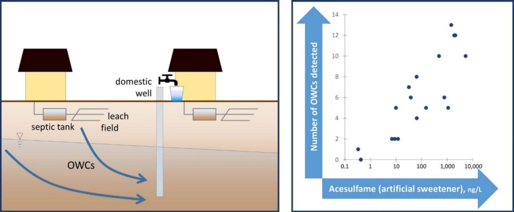
Figure 1-3. Conceptual model of drinking water contamination by neighboring organic wastewater compounds (OWCs) and use of sweetener as indicator of potential number of contaminants detected.
Source: Schaider et al. 2016. Open Access, https://creativecommons.org/licenses/by-nc-nd/4.0/
Contamination of groundwater with PFAS from DSS is a challenge in site characterization projects given that the operation of domestic leach fields and the variety of consumer products that contain PFAS can lead to areas of diffuse contamination from wastewater sources. Examples of DSS can include leach fields and seepage pits, depending on local subsurface and environmental conditions. The presence of PFAS in consumer products, including cosmetics, cleaning products, cookware, carpets, upholstery, electronic products (Glüge et al. 2020), and certain foods (Hill et al. 2022; Lasters et al. 2022; Mikolajczyk et al. 2022; Ghisi et al. 2019; Lupton et al. 2014), can result in PFAS in household wastewater. Much like wastewater at public treatment plants, it should be expected for domestic wastewater to contain PFAS (MacMahon et al. 2022; Schaider et al. 2016).
It is important to emphasize that the existence of a significant statistical correlation between the levels of PFAS and markers such as sweeteners or pharmaceuticals and personal care products in private water supply wells does not eliminate the possibility that other sources of PFAS could also be contributing to the contamination. For example, Schaider et al. (2016) were not able to rule out potential influence from landfills in their conclusions. In fact, artificial sweeteners have been used to evaluate the impact of landfills on groundwater (Propp et al. 2022), and artificial sweeteners (Li et al. 2021) and pharmaceuticals (Kinney and Vanden Heuvel 2020) have been found in biosolids used on agricultural fields.
Other sources that could contribute to PFAS in groundwater or water supply wells have been documented. For example, Sivaram (2022) noted the presence of PFAS in commercially available garden soil mixes and composts, and at least one study documented downward migration of PFAS from compost (Saha et al. 2024), indicating that composts or other lawn and garden amendments have the potential to contribute PFAS to groundwater. PFAS contamination could also originate from a variety of diffuse sources such as wet precipitation (Pike et al. 2021) and dry deposition (Schroeder et al. 2021) that may infiltrate and percolate, transferring from the atmosphere into the vadose zone and groundwater (Guo, Zeng, and Brusseau. 2020). In addition, because the mix of consumer products used in a household or business can vary, the mixture of PFAS, or PFAS signature, should not be expected to be similar for all septic sources. Because of these potential complications and uncertainties, a multiple-lines-of-evidence approach should be used when investigating septic systems as potential PFAS sources.
1.3.3 Perfluoroalkyl Acids Precursor Biotransformation
This section presents information on precursor biotransformation to perfluoroalkyl acids (PFAAs). It builds upon Section 5.4.2, which introduced perfluoroalkyl acid (PFAA) precursors, and Section 5.4.4.2 and Section 5.4.4.3, which discussed aerobic and anaerobic biological pathways, respectively. The introduction discusses why it is important to understand PFAA precursor biotransformation and provides background information on the process. This is followed by detailed information on the development of a precursor transformation database, and a short discussion on the application of PFAA precursor data.
1.3.3.1 Introduction
Some PFAS, commonly referred to as precursors, can undergo biotransformation processes, leading to the formation of degradation products and, ultimately, the terminal products of perfluoroalkyl acids (PFAAs). Understanding the transformation pathways and kinetics helps in predicting how PFAS mixtures change over time and how they travel and persist in different environmental media. This section describes PFAS biotransformation and the process of compilation of a database of precursor degradation rates. Please refer to Section 2.2.2 for descriptions of PFAS nomenclature and PFAS groups and Section 5.4 for discussion of transformation processes. Although Table 4-1 is meant to be a compilation of biodegradation rates, not all studies described in Table 4-1 have controls that definitively exclude the potential for abiotic transformation within the experiment. Additionally, not all studies had controls that excluded additional removal processes such as sorption.
Understanding the accumulation of PFAAs through biodegradation is important from a regulatory and risk assessment perspective. The mobility, toxicity, and bioaccumulation tendencies of terminal products appear to differ from the parent substances, and, as such, understanding the occurrence, diversity, and complexity of transformation pathways has become a priority in the assessment of PFAS risk. Consequently, documenting the current understanding of the number and types of transformation products, both terminal and intermediate, as well as the rates at which they are generated and transform, is an essential endeavor.
Additionally, the biological conversion of precursors can be impacted by remediation activities such as aeration in groundwater in the proximity of biosparging or air sparging wells (McGuire et al. 2014) or chemical oxidation (Houtz and Sedlak 2012). Understanding precursor transformations can also help in the assessment of appropriate remedial actions by enabling forecasts of transformation rates of various PFAS and enabling the quantification of “chemical retention” of PFAA precursors (future PFAAs) in a system alongside the geochemical retention of PFAAs through standard processes such as sorption or matrix diffusion (Newell et al. 2021). Collectively, the management of these retention processes is referred to as PFAS monitored retention (Adamson et al. 2025).
For further context, in most cases, cationic and zwitterionic PFAS tend to be retained in soil, whereas anionic PFAS exhibit greater mobility and are more likely to migrate into groundwater (see Section 5). Given that a significant proportion of zwitterionic and cationic PFAS are precursors—and considering that their retention in soil is not permanent—it is critically important to understand their transformation pathways and environmental fate. Further investigation into the fate and transport of zwitterionic and cationic PFAS is essential for assessing long-term contamination risks and developing effective remediation strategies (Tajdini et al. 2025)
Some studies of PFAS precursor biodegradation have focused specifically on PFAS present in AFFF. The study of PFAS transformation within AFFF sources has aided understanding of PFAS biodegradation pathways. Studies have shown that the pathways depend on the different source profiles produced by different AFFF production methods (for example, electrochemical fluorination [ECF] or fluorotelomerization, with precursors from these processes shown to degrade into perfluoroalkyl acids (PFAAs) as one of their terminal environmental products (Liu et al. 2021). To aid in general understanding of AFFF biodegradation pathways, some researchers have further classified precursors into primary and secondary ECF- or fluorotelomerization-based precursors. Primary precursors are those that were originally incorporated into AFFF formulations as intended PFAS components and are typically present at high concentrations. Secondary precursors, alternatively, are intermediate transformation products (excluding PFAAs) derived from primary precursors and are commonly detected in AFFF-impacted environments (Yan et al. 2024).
Awareness of complex PFAS precursor transformation pathways to intermediates and end products provides important context for understanding PFAS fate and transport. Development of reactive fate-and-transport models to predict the movement and behavior of PFAS in soil, water, air, and biota will require and benefit from enhanced understanding of biotransformation pathways and kinetics. By accounting for the diversity of transformation pathways and kinetic parameters, these models can provide more accurate assessments of PFAS behavior and environmental distribution.
1.3.3.2 Development of Precursor Transformation Database
The need for compilation of available precursor transformation kinetics was identified for practitioners to reference or use as guidance. A centralized table curated from peer-reviewed published literature was developed and presented as a tab named Biotransformation in Table 4-1 to address this need.
Sources of data on transformation of PFAS in soil media were examined, giving priority to peer-reviewed scientific literature due to the vetted nature, traceability, and thus reliability of such data. All references are included in the References tab of the table. While the data presented in Table 4-1 are the current state of the science, the values are highly dependent on the experimental conditions. Study- or site-specific information extrapolated from Table 4-1 to other situations may lead to erroneous assumptions of PFAS transformation rates and extent. Importantly, interested parties must be cautious about comparing half-lives or rate constants from different studies and using literature values from specific studies for other purposes. Additionally, some of the values are true biodegradation rates while others are based on source decay or release. For these reasons, the rate constants and related values presented in Table 4-1 should be considered estimates, since derivation of these parameters is sensitive to experimental conditions, substrates, and analytical error (since standards are not available for many precursors and daughter, intermediate, and downstream products).
Data Collection Method
Table 4-1 presents only papers in which a transformation rate or half-life was explicitly reported and thus does not represent the full extent of the published information on PFAS biotransformation. Table 4-1 includes biotransformation pathways and kinetics for PFAS from a variety of sources, including AFFF. To access a detailed description of foam formulations and a compilation of PFAS frequently present in AFFF, please refer to Section 3. Section 2.2.2, and Figure 2-5, include information about the PFAS family and different groups and subgroups of PFAS.
The columns in Table 4-1 include categories such as parent PFAS name, average atomic weight, primary daughter product(s), intermediate metabolites, downstream products (downstream metabolites, term defined and discussed below), the matrix in which the precursor transformation experiments or observations were completed, the period of observation (defined as assay length), geochemical condition under which the transformation rates were observed, the transformation kinetics information identifying if the values are half-lives or rate constants, and published literature references. Numerous studies in the scientific literature provide qualitative descriptions of transformation pathways and product accumulation; however, they were not included in this compilation because they do not explicitly report transformation rates or half-lives. Additionally, many studies present precursor transformation data—such as concentration versus time plots—without calculating or reporting a rate or half-life. These studies were also excluded from the database.
Perfluoroalkyl Acids Precursors in Table 4-1
The following 13 groups of PFAA precursors will be discussed for precursor transformation:
- fluorotelomer carboxylic acids (FTCAs)
- fluorotelomer sulfonic acids (FTSAs)
- perfluoroalkane sulfonamides (FASAs)
- perfluoroalkane sulfonamidoethanols (FASEs)
- perfluoroalkane sulfonamido acetic acids (FASAAs)
- fluorotelomer alcohols (FTOHs)
- polyfluoroalkyl phosphate esters (PAPs)
- polyfluoroalkyl amine oxides (PFNOs)
- perfluoroalkyl ether carboxylic acids (PFECAs)
- perfluoroalkyl ether sulfonic acids (PFESAs)
- other perfluoroalkyl compounds
- polyfluoroalkyl ether acids
- polymer mixtures
In addition to the above groups, there are some studies listed that report degradation of perfluoroalkyl acids, although most of these values are NDO (no degradation observed). The environmental matrix considered was primarily soil. However, if high-quality data were available in other media, including activated sludge and sediment, they were also recorded. Experimental conditions included both aerobic and anaerobic systems, but most data were obtained under aerobic conditions.
Of the 13 different groups listed above, limited information was available for four groups, namely FASAs, FASAAs, FTOHs, and PAPs. Additional research is needed for precursor transformation rates.
Transformation Product Categories
The sequence or network of transformation products was split into different categories:
- intermediate products
- daughter products
- downstream products (downstream metabolites)
- terminal products
Intermediate products: Intermediate products were identified as detected compounds present in the transformation pathway between the parent and daughter product for which the reaction rate or half-life was reported. In cases where the intermediate product was reported, the authors determined the rate constant or half-life through the measured accumulation of the specified daughter product.
Daughter products: The daughter products were those determined to represent the reported rate constant or half-life at the authors’ discretion. Many papers were not explicit and reported the reaction rates in relation to the removal of the parent compound but not in relation to the formation of a specific daughter compound. In these instances, the first measured compound identified in the transformation pathway resulting from the measured decrease in concentration of the parent/precursor compound was considered a daughter product. In some cases, the metabolic pathways were not singular and multiple daughter products were possible. In these instances, more than one daughter product was listed.
Downstream products: Downstream metabolites were any compounds detected as degradation products further along the reported pathway than the daughter product. Some papers reported molar yields or relative concentrations of multiple metabolites detected. This information was included in the table where available. PFAAs were the most frequent terminal products. However, given that many of the studies did not continue until complete transformation of the parent compounds, the publications identified partial degradation of compounds at different points along the transformation pathway. Relative concentrations of downstream metabolites documented a time-specific extent of transformation in the degradation pathway.
Terminal products: Terminal products are a subset of downstream metabolites after which there is most likely no further transformation. They are most often PFAAs. A few studies that investigated PFAAs as parent compounds and observed no further degradation have also been included in Table 4-1, providing additional support for the characterization of PFAAs as terminal transformation products.
Transformation Kinetics
Transformation kinetics data for the precursor/parent PFAS and transformation products such as reaction rate constants and half-life estimates were mined from sources whenever available. Liu and Liu (2016) found a negative correlation between the half-lives and corresponding molecular weights of 11 PFAS that undergo biotransformation in aerobic soils. This indicates that molecular weight may serve as a reliable indicator of the overall stability of low molecular weight PFAS that have shorter carbon-fluorine chains in aerobic environments. To provide a standardized frame of reference, whenever only either the rate constants or the half-life values were provided, the other value was calculated assuming the transformation reaction followed a first-order kinetics model. This occurred unless otherwise indicated in the study. Additionally, a few studies reported no observable degradation for certain PFAS; in these cases, the kinetic data were recorded as no degradation observed (NDO). Importantly, reaction rates depend on factors such as temperature, pH, oxidation-reduction potential, moisture content, and similar parameters. Kinetic values should be considered site-specific and may vary over time. The reaction rates presented in Table 4-1 are intended to provide a general understanding of which products are likely to prevail during transformations.
Transformation Conditions
Most reported transformations occur under aerobic conditions, which favor oxidizing reactions. Under anaerobic conditions, PFAAs are not always formed (Section 5). Experimental (or field) conditions such as temperature, pH, test duration, soil type, and test settings (for example, microcosm, culture) are recorded in Table 4-1. Transformation has been observed with multiple soils (except for some sulfonamide precursors), usually in presence of alternate organic substrates (for example, glycols in AFFF, acetate, glucose), suggesting some of the transformations may be catalyzed by microorganisms using these primary substrates via nonspecific oxygenases with cometabolic pathways for PFAS transformation (Yang et al. 2022; Olivares et al. 2022; Ruyle et al. 2023). Some studies have also reported the role of sulfur limitation in fluorotelomer transformation (Van Hamme et al. 2013).
1.3.3.3 Applications
The present envisioned uses for this type of PFAA precursor transformation data include:
- mapping of observed and traceable degradation pathways for contaminant forensics and fingerprinting
- introduction of reliable input variables for reactive transport models
- PFAS exposure assessments in which both PFAA precursors and PFAAs are present in the environment or within organisms for bioaccumulations models (Glaser et al. 2021)
- development of a baseline for prioritization of exposure and toxicity studies
- development of site-specific degradation rate estimations
As regulations continue to evolve to address PFAS impacts, including diverse transformation pathways in risk assessments is important to ensure regulatory compliance and design effective mitigation strategies. Understanding the full spectrum of PFAS transformation pathways helps regulators, remediation practitioners, and local infrastructure decision makers and operators to set appropriate guidelines and timeframes for PFAS management and remediation efforts. Accurately clarifying the diversity and complexity of PFAS transformation pathways in fate-and-transport modeling is essential for a comprehensive understanding of the environmental impact, human exposure risks, and regulatory implications associated with these persistent chemicals.
1.3.4 Groundwater Partitioning, Colloidal Transport, GW-SW Interactions
The following supplements Section 5.2.5 and Section 5.3.4 by further discussing the fate and transport of PFAS in groundwater and the effects of co-contaminants, colloidal transport, and groundwater-surface water interactions.
1.3.4.1 Co-contaminant Effects on Fate and Transport
In addition to the effects of aqueous chemistry and soil interactions, PFAS fate and transport may be affected by the presence of co-contaminants. Section 5.2.5 provides a discussion of interactions between PFAS and co-contaminants, including light nonaqueous phase liquid (LNAPL). Key interactions are as follows:
- LNAPL may contribute to PFAS retention via phase partitioning or interface accumulation; where only residual (immobile) LNAPL is present, LNAPL may contribute to a reduction in PFAS flux.
- PFAS accumulation at the LNAPL/water interface is likely to be less than accumulation at the AWI.
- LNAPL biodegradation can deplete oxygen, causing a local transition from aerobic to anaerobic conditions, which may affect the transformation of PFAS precursors.
Ongoing research continues to provide additional insights into PFAS interactions with co-contaminants. Multiple studies have evaluated relative effects of phase partitioning and interface partitioning in water-LNAPL systems, and many of these studies have involved calculation of partition coefficients for both processes. These studies have generally involved only a single co-contaminant (or a small number), whereas real-world scenarios involving multicomponent mixtures of PFAS and LNAPL (or other co-contaminants) are limited. In general, PFAS retention due to interface partitioning is reported to be greater than retention due to partitioning into bulk nonaqueous phase liquid (NAPL) phases. An overview of these studies is provided in the remainer of this section.
It should be noted that the authors of these studies use slightly different definitions for the terms and coefficients they present. Generally, three terms are commonly used: solid-phase partition (absorption) coefficient, Kd; NAPL-water partition (absorption) coefficient, Kn; and NAPL-water interface adsorption coefficient, Knw. Interface adsorption may also be referred to as interfacial adsorption or accumulation. “Partition coefficient” may be used as a general partitioning term (K) or may be used to describe media-specific partitioning (for example, Kd). In some instances, the term “sorption coefficient” is used to describe absorption or adsorption if the precise nature of the partitioning is not determined.
Christie et al. (2023) explored the need to account for residual LNAPLs at AFFF-impacted sites as potential sources of PFAS contamination. Though interface accumulation was not studied, insights into AFFF formulations and occurrence in groundwater were provided. The research group evaluated PFAS in bulk LNAPL from groundwater monitoring wells at military AFFF sites, using targeted and non-targeted analytical methods for anionic and neutral PFAS (that is, fluorotelomer alcohols). PFAS were detected in most LNAPL samples, with most frequently detected compounds including PFOS (nondetect to 11,100 ng/L) and perfluoroalkyl sulfonamides, such as perfluorohexanoic acid (PFHxSA) (nondetect to 67,700 ng/L). Insights were provided into the source AFFF, with some samples showing signatures of various AFFF formulations (for example, ECF versus fluorotelomerization). The analysis evaluated bulk LNAPL and did not evaluate interface accumulation. The presence of residual LNAPLs at AFFF-impacted sites should be factored into the planning and execution of remediation strategies.
Fang et al. (2024) explored the partitioning of PFAS in LNAPL; they found that PFAS partitioning was significantly influenced by both the structure of PFAS and the characteristics of LNAPL, with LNAPL potentially serving as a transport reservoir. The team investigated the partitioning of six PFAS (PFBA, PFOA, PFBS, PFOS, 6:2 FTS, and 8:2 FTS) into a weathered, field-collected LNAPL. Individual partition coefficient (K, defined as ratio of LNAPL concentration to aqueous concentration) values were determined via batch experiments. The study showed that 1) K values increase with increasing perfluorocarbon chain length; 2) K values increase with greater C-F to C-H bond ratios; and 3) the structure of the head group did not strongly affect the K values. In all cases, a higher initial aqueous concentration of LNAPL resulted in a greater K value. The study demonstrated that batch experiments may be useful for determining LNAPL/aqueous partition coefficients for PFAS. Similar to Christie et al. (2023), this analysis evaluated bulk LNAPL and did not evaluate interface accumulation.
Ding et al. (2022) evaluated interaction between PFAS and chlorinated volatile organic compound dense nonaqueous phase liquid (DNAPL) associated with a fluoropolymer manufacturing facility. Chlorinated volatile organic compounds present at the site include dichloromethane, trichloromethane, 1,1,2-trichloroethane, carbon tetrachloride, trichloroethene, and tetrachloroethene (PCE). Seventeen target PFAS were analyzed, including select PFCAs, PFSAs, and precursors. Laboratory experiments and field samples were evaluated to calculate sorption coefficients (referred to by the authors as Kd). In field samples, elevated PFAS concentrations were detected in groundwater, with PFOA as high as 204 μg/L. Laboratory experiments showed that the presence of DNAPL caused the Kd values for nearly all PFAS to increase. The values increased with an increase in carbon chain length, with the Kd for PFOA increasing by a factor of nearly 4 in the deep aquifer (where DNAPL was inferred to be present). Similar to the studies discussed above, no investigation was made between absorption of PFAS into the bulk DNAPL versus adsorption of PFAS to the water-DNAPL interface.
Liu et al. (2024) evaluated the impact of heterogeneous LNAPL on PFAS transport via a laboratory study comprising two-dimensional (2-D) flow cells. Decane and PFOS were used as model NAPL and PFAS, respectively. Two flow regimes were created, one with NAPL in residual saturation and a second with NAPL in greater than residual (pool) saturation. An influent PFOS concentration of 30 mg/L was used to represent concentrations found in source zones. The method of temporal moments, a commonly used method for analyzing concentration breakthrough curves by comparing theoretical moments of concentration to breakthrough data (Pang et al. 2003), was used to calculate retardation factors, including the effects of solid-phase adsorption, NAPL-water interfacial adsorption, and absorption into bulk NAPL. The Kn value for PFOS in decane was measured at 0.02. The retardation factor in the NAPL residual saturation flow cell measured by moment analysis was 1.7, with solid-phase adsorption, NAPL-water interfacial adsorption, and NAPL absorption being 0.56, 0.43, and 0.1, respectively. The retardation factor in the NAPL pool flow cell measured by moment analysis was 1.4, which was attributed to minimal contribution to retardation by NAPL-water interfacial adsorption due to flow bypass. In 3-D numerical simulations, the retardation factors varied from 1.13 to 2.65, with higher values being associated with closer proximity to the NAPL source zone. Therefore, the spatial distribution of LNAPL likely influences PFAS mobility, retardation, and occurrence of potential preferential pathways for PFAS transport.
Van Glubt and Brusseau (2021) studied PFAS retention by NAPL partitioning and interface adsorption, as well as the effect of PFAS on NAPL mobilization and distribution. PFAS aqueous solutions contained PFOS, PFOA, or PFPeA (perfluoropentanoic acid), while decane and trichloroethene (TCE) were used as NAPLs. Batch and column experiments were used to determine partitioning of PFAS into the bulk NAPL phase and PFAS transport in the presence of residual NAPL. Batch solubilization experiments were conducted to investigate the effect of PFOS concentrations on the aqueous concentration of TCE. Column experiments were also used to determine whether PFAS could cause NAPL mobilization. Batch experiment-derived Kn values for PFOS were 0.11 in TCE and 0.022 in decane, while batch experiment-derived Kn values for PFOA were 0.19 in TCE and 0.065 in decane. For NAPL-water interfacial tension, the activity was observed to increase with carbon chain length. Other factors influencing Kn values include the protonation/deprotonation status of the PFAS, as described by the pKa value. Overall, the Kn values for PFOS and PFOA are small compared to other NAPLs. Retardation factors for PFOS in columns with TCE NAPL ranged from 2.5 to 3.3, while for decane NAPL they ranged from 1.7 to 2.6. The retardation factor for PFOA in a column with TCE NAPL was 1.5. However, the contribution of partitioning to the bulk NAPL phase was minimal for all these experiments, ranging from 0.5% to 19% of total retention. The results of Van Glubt and Brusseau (2021) also suggest that PFAS typically only significantly affect NAPL solubilization and mobilization when present at high concentrations (hundreds of milligrams per liter) that are rarely observed at legacy AFFF source-zone sites but may apply to both recent AFFF releases and historical-release situations.
Kosteleros et al. (2021) performed laboratory studies looking at the effects of LNAPL (jet fuel) on AFFF mobility in the vadose zone. These studies were conducted on five AFFFs and one fluorine-free foam using phase behavior and column experiments. The latter were performed to mimic AFFF migrating through the soil column and encountering LNAPL. The outcomes found that there was the formation of a microemulsion that had a higher viscosity than either the LNAPL or the AFFF and was immobile and stable in the laboratory for at least one year. The result also showed that the LNAPL was a sink for the surfactants/PFAS associated with AFFFs. No conclusions were generated concerning the long-term stability in the environment of the microemulsion, including binding the PFAS/LNAPL in place. Nor was there an evaluation of impact on the biodegradation rate of the LNAPL.
Liao et al. (2022) investigated the effect of residual NAPL on transport and retention of individual PFAS and PFAS mixtures. The six PFAS employed were PFBS, PFHxS, perfluoroheptanoic acid (PFHpA), PFOA, PFOS, and perfluorononanoic acid (PFNA). Tetrachloroethene (PCE) was chosen as the NAPL. Interfacial tension measurements were conducted with PCE NAPL and aqueous-phase PFAS, and batch reactor experiments were used to assess PFAS partitioning into PCE NAPL and adsorption on the solid phase. Column experiments were performed to investigate the impact of residual PCE NAPL on PFAS transport in a quartz sand, and a mathematical model was developed to account for PFAS accumulation at the NAPL-water interface and partitioning into the NAPL and solid phases. PFAS partitioning into PCE NAPL was linear. The PFOS NAPL-water coefficient Knw was 0.098, while the PFNA NAPL-water coefficient Knw was 0.048. The NAPL-water coefficient Knw for PFOA, PFHpA, PFHxS, and PFBS in a mixture ranged from 0.028 to 0.034. There was a minimal effect on partitioning values due to the PFAS being in a mixture. The sand mixture was found to have a low adsorption capacity for PFAS in column experiments. Column experiments were then performed with a residual PCE saturation of 16%, using PFOS and PFNA. These experiments showed a delay in peak arrival times, with NAPL-water interfacial accumulation accounting for 83% and 88% of the retardation for PFOS and PFNA, respectively. In contrast, PFBS, PFHpA, PFHxS, and PFOA were only slightly delayed in their breakthrough, showing that they minimally accumulate at the NAPL-water interface. Also, the effect of PFAS on PCE solubility was minimal over a PFAS concentration range from 0.01 to 10 mg/L.
Costanza et al. (2020) focused on NAPL-water and air-water interfacial tension values for PFOA, PFOS, perfluorooctane sulfonamide (FOSA), and AFFF formulations at concentrations from 0.1 to 1,000 mg/L. NAPLs tested included jet fuel, PCE, and dodecane. Interfacial tensions were measured for both air-water and NAPL-water experiments. Of note are the calculations performed for the mass of PFOA, PFOS, and FOSA in the aqueous phase, adsorbed to soil, and at the air-water and dodecane-water interfaces for a sandy soil. These results showed that for concentrations below 1 mg/L, most of the mass of PFOA, PFOS, and FOSA is at the AWI, and little is at the dodecane-water interface with a dodecane saturation of 2%. This study highlighted the importance of PFAS accumulation at the AWI in assessing mass transport of PFAS in aqueous systems.
Brusseau (2018) proposed a comprehensive conceptual model for PFAS retention and transport in porous media systems. Literature was searched for physicochemical property data, including phase-distribution coefficients, for PFOA and PFOS, which were then used to calculate retardation factors. Each of the phase-distribution coefficients contributes to the combined retardation factor in a porous media system, including air-water partitioning, adsorption at the AWI, adsorption to the solid phase, NAPL-water partitioning, and adsorption at the NAPL-water interface. Assumptions in the conceptual model included the insignificance of gas phase transport relative to aqueous-phase transport (thereby making volatilization to the gas phase a retention process), and that NAPL is immobile and has a minimal impact on solid surfaces in terms of blocking solid phase adsorption. A sandy quartz vadose zone soil with moderately low organic content, a water saturation of 78%, a NAPL saturation of 2%, and an air saturation of 20% was assumed. PFOA, PFOS, and 8:2 fluorotelomer alcohol (a precursor to PFOA and other PFCAs such as PFNA and PFHpA) were included. Partition coefficients were gathered from the literature. Notably, reported Kow values were used as a surrogate for Knw partition coefficients. For PFOA and PFOS, the contribution of NAPL-water partitioning was small: for PFOA, the total retardation factor was 14.1, with NAPL-water partitioning contributing 16%; for PFOS, the total retardation factor was 47.9, with NAPL-water partitioning contributing 8.2%. For both PFAS, the dominant contributor to retardation was air-water interfacial adsorption. For FTOH, however, NAPL-water partitioning contributed 98% to the total retardation factor of 9,906. This study (Brusseau 2018) did not involve any laboratory or field aspects. It is important to note that the Kow values used as surrogates for Knw values ranged from 83 (PFOA) to 282 (PFOS) to 380,189 (FTOH). It is important to better understand the Knw for FTOH given its role as a PFOA precursor. Last, because the model developed by Brusseau (2018) was based on the available literature at the time, more recent literature should be used for the partition coefficients of the subject PFAS if the model is to be used. Table 1-6 summarizes the partition coefficients in this section.
Table 1-6. Summarized PFAS:NAPL partition coefficients (based on references in this section).
| PFAS | Weathered LNAPL | Decane | TCE | PCE |
|---|---|---|---|---|
| PFBA | 0.02 to 0.22 | |||
| PFBS | 0.06 to 0.33 | 0.0291 | ||
| PFOA | 7.485 to 9.034 | 0.02
0.0651 |
0.191 | 0.0321 |
| PFOS | 11.65 to 38.8 | 0.0221 | 0.111 | 0.098 |
| 6:2 FTS | 1.11 to 1.52 | |||
| 8:2 FTS | 18.69 to 19.10 | |||
| PFNA | 0.048
0.0402 |
|||
| PFHpA | 0.0276 | |||
| PFHxS | 0.0340 |
1 Batch NAPL-partitioning experiment values from Van Glubt and Brusseau (2021).
1.3.4.2 Colloidal Transport of PFAS in Groundwater
Colloid and colloid-facilitated solute transport have been investigated in the subsurface in recent years. Deb and Chakma (2023) “identified fundamental mechanisms of colloid mobilization and the principal mathematical relationship describing colloid transport including attachment-detachment, size exclusion, and air-water interfacial area.” The paper also considered mobile colloid attachment at the AWI and the air-water-solid contact line present during infiltration and water table fluctuations.
Bierbaum et al. (2023) investigated the sorption processes that affect PFAS transport during leaching by creating a continuum model and a particle tracking model and comparing results to data from previously conducted column and lysimeter experiments. The authors proposed that colloid-facilitated transport in column and lysimeter experiments resulted in “premature leaching” of PFOA and PFOS. Sorption processes investigated included equilibrium and rate-limited sorption to soil and AWIs, and colloid-facilitated transport. The study highlighted that precursor transformation may be more relevant for long-term leaching of PFAS in the environment compared to rate-limited sorption, and that AWI sorption has the potential to be the dominant retention mechanism at PFAS-contaminated sites. The authors also noted that results of the model simulations suggest that “premature leaching” may be a result of colloid-facilitated transport, and that this mechanism appears to be more significant for PFOS than PFOA, likely due to the increased sorption affinity of PFOS compared to PFOA.
Borthakur et al. (2021) noted that flow interruptions from groundwater injection in clay-rich soil caused increased leaching of PFBA and PFOA associated with increased soil colloid concentrations. Concentrations of PFOA were higher than PFBA in effluent samples, indicating that colloid transport is more significant for long-chain PFAS due to their higher sorption affinity. This was corroborated in a series of column studies by Das et al. (2024) to simulate managed aquifer recharge, which showed that a greater fraction of PFOS in the effluent was associated with particulates compared to PFBS, which was predominantly in the dissolved phase. The authors noted that colloids may play a higher role in PFAS transport in conditions that release colloids (Borthakur et al. (2021), which could include natural fluctuations in groundwater flow, extreme precipitation events, or soil disturbance.
Microplastics are often associated with PFAS and can be transported as colloids (see Section 1.8.4).
1.3.4.3 Groundwater–Surface Water Interactions
Understanding the fate and transport of solute contaminants at the groundwater-surface water interface is an important component of site characterization and CSMs (see Section 16.7). This interface (also known as the hyporheic zone) consists of saturated sediments comprising streambeds, stream banks, and floodplains that exist between surface water and underlying/laterally adjacent aquifer materials. Section 5.3.4.1 discusses PFAS in the hyporheic zone in the context of how changing redox conditions can affect biodegradation. This section provides information for additional topics and references.
Bed sediments often have different physical and chemical characteristics relative to the aquifer itself. These characteristics include:
- reduced hydraulic conductivity associated with silt and clay (discretized as a zone of reduced “conductance” in groundwater flow models)
- increased organic carbon content
- changes in geochemical parameters (redox, solute concentrations)
- presence of biota
- brackish, saline, and tidally influenced conditions in coastal areas
As discussed in Section 5.2.3, sorption of PFAS can be influenced by a variety of factors, including grain size, organic carbon (OC), presence of co-contaminants, and carbon chain length of the PFAS molecule. In general, the characteristics of the hyporheic zone would tend to inhibit PFAS flux in groundwater by reducing seepage and enhancing sorption to OC.
In coastal areas, PFAS sorption to the aquifer or sediment matrix is enhanced by the ionic strength of brackish or saline water. Early in the progression of PFAS research, Chen et. al (2012) noted that sorption of PFOS to marine sediments was strong—approximately 10 times higher than that in fresh water. The sorption affinity was well correlated with the sediment OC content, confirming the significance of hydrophobic interactions. This phenomenon is more recently referred to as “PFAS salting out,” defined by Hort et al. (2024); (see Section 1.3.5.1 for more details on the salting-out effect), which becomes an increasingly dominant process as “PFAS in fresh groundwater mixes with saline groundwater near marine shorelines, resulting in increased sorption to aquifer solids” (Hort et al. 2024).
Studies that directly explore PFAS behavior at the groundwater–surface water boundary are sparse, with some authors calling for more research in this area (Divine et al. 2023). Tokranov et al. (2021) examined the impact of groundwater–surface water boundaries on PFAS transport and transformation in a flow-through lake, fed by contaminated groundwater, and its downgradient surface water–groundwater boundary. PFAA precursors made up 45% of the total PFAS concentration in the oxic lake, which was impacted by a fire training area and historical wastewater discharges. In shallow porewater downgradient from the lake, the proportion of PFAA precursors decreased by 85%; the decrease was attributed to enhanced precursor transformation at the boundary between surface water and groundwater. Tokranov et al. (2021) also explored the effect of seasonality on both sorption capacity and transformation rates in the hyporheic zone. The study noted increased PFAA concentrations in the hyporheic zone and in groundwater downgradient of the lake in winter months, showing an inverse correlation with temperature (increased PFAA with decreased temperature) and a strong inverse correlation with nitrate. Seasonal changes could not be explained by precursor transformation or AWI sorption. The authors noted large temporal variations in field-derived Kd values and suggested that future work should investigate whether there are biological mechanisms driving sorption. Tokranov et al. (2021) conclude that biogeochemical conditions at the groundwater-surface water interface result in complex and competing transport and transformation processes.
Given the large number of variables affecting PFAS interactions in the hyporheic zone, practitioners may find it advantageous to collect site-specific data. In these instances, several tools exist to characterize site-specific partitioning of PFAS to the range of media and phases and to measure flux of PFAS between groundwater and surface water. These include drive-point piezometers, porewater samplers (USEPA 2023), seepage meters, tide charts, stilling wells (gauged or with pressure transducers), sediment cores, and biological tissue sampling.
PFAS passive samplers are also becoming available for deployment in sediments at the groundwater-surface water interface that allow for discrete, time-weighted sampling and the assessment of PFAS distribution and flux (Eldridge et al. 2025; Carter et al. 2025). See also the ITRC “Passive Sampling Technology Update” (ITRC 2024).
1.3.5 Understanding PFAS in Marine Environments
This section describes some of the key factors affecting the fate of PFAS in transport from fresh water to the marine environment, in ocean spray via aerosolization and in ocean foam, as well as the bioaccumulation of PFAS to marine life. This topic supplements Section 16 and Section 5.3.4, which address PFAS in a freshwater environment.
1.3.5.1 Salting-Out Effect
An important factor influencing the behavior of PFAS at the freshwater/marine water interface is the salting-out effect. As discussed below, the solubility of PFAS decreases in the presence of elevated salinity in water (that is, high cation and anion concentrations), and PFAS has a higher tendency to sorb to solid-phase materials. This process has the potential to increase retention of PFAS in saline environments. This phenomenon was observed by Munoz et al. (2017) in a survey of PFAS in an estuary discharging to the Atlantic Ocean in France. These authors observed an increase in the affinity of PFAA compounds to particulate matter in the presence of increasing saltwater concentrations. Using field data, these authors derived sorption coefficients based on both particle concentration and salting-out effects for C7–C9 PFCAs and C6–C8 (branched and linear) perfluoroalkane sulfonic acid (PFSA).
Yin et al. (2022) conducted a series of PFAS sorption/desorption studies at different salinities using marine sediment collected from the South China Sea. The results showed that the sorption coefficient increased with increasing PFAS chain length and salinity, indicating that hydrophobic and electrostatic processes are involved. In a literature-based study of PFAS in groundwater plumes discharging to sandy beaches, Hort et al. (2024) used a multivariate regression model developed from data at three PFAS sites to estimate the increased sorption of PFOS with ionic strengths as follows:
- low ionic strength (< 10 ppt), estimated a 1- to 2.5-fold increase in PFOS sorption
- medium ionic strength (10 to 20 ppt), a 2- to 6.4-fold increase in PFOS sorption
- higher ionic strength (> 20 ppt), a 3.8-fold to 25-fold increase in PFOS sorption
In an earlier study, López-Fontan et al. (2005) demonstrated the gradual micellization (self-aggregation) of sodium perfluorooctanoate (SPFO) in water with increasing ionic strength. At low ionic strength (0.01 mol decimeter–3 [dm]–3), pre-micelles of perfluorooctanoate ions are formed. At 0.02 mol dm–3, sodium ions (Na+) are captured and form micelles at a critical micelle concentration of 0.03 mol dm–3. At the critical micelle concentration, the micelles are significantly ionized. At around 0.06 mol dm–3, the degree of ionization was lower, suggesting the micelles are more compact.
Other studies have found that the type of cation present in the saltwater environment can influence the salting-out effect. In a series of isotherm studies, Steffens et al. (2021) found that divalent cations such as Ca2+ and Mg2+ resulted in more surface aggregation (accumulation at the air-water interface, see Section 4.2.8) and bulk aggregation (formation of micelles see Section 4.2.7) of PFOS at lower ionic concentrations compared to monovalent cations such as Na+ and K+. Similarly, column experiments by Li et al. (2021) showed that an increase in ionic strength led to greater retardation of PFOA in unsaturated columns, and that Ca2+ resulted in greater retardation than Na+. Using a mass-action model to determine the impact of monovalent versus divalent salts on the air-water partitioning coefficients for PFOA, Le et al. (2022) also found that divalent cations had a much larger impact on increasing the air-water distribution coefficient of PFOA than monovalent cations. An earlier column study by Lyu and Brusseau (2020) noted that while PFOA retardation was affected by changes in ionic strength under unsaturated conditions, the impact was minimal under saturated conditions—emphasizing the importance of the AWI to adsorption and retardation.
Based on literature, Hort et al. (2024) identified conceptual mechanisms for the retention of PFAS in groundwater and saturated soils with high salinity: neutralizing surface charge; salting out process leading to: increased sorption to solids and increased AWI sorption; bridging by divalent cations, leading to increased sorption to solids; and, increased formation of micelles from increased cation concentrations.
Last, several studies have shown that the type of PFAS also influences the salting-out effect and the retention of PFAS. For example, Yin et al. (2022) showed that the sorption of PFCAs on marine sediments was lower than PFSAs with the same chain length, and PFOS showed much stronger sorption than 6:2 FTSA. As discussed by Steffens et al. (2021), although the PFAS C-F bond exhibits low polarizability (see Table 4-2), the functional head of individual PFAS (for example, carboxyl, sulfonate) governs the extent of polarizability (see Section 2.2.3). Others cited by Steffens et al. (2021) have shown a higher polarizability of PFOS than of PFOA, resulting in greater increases in Kd values for PFOS compared to PFOA in increasingly saline solutions.
In a series of column leaching studies using different soils contaminated with AFFF, Tsou et al. (2024) demonstrated that the type of PFAS has an influence on its fate in a saltwater environment. These authors found that PFOA moved through the columns faster than other PFAS analytes tested (PFOS and two precursors) at all water salinities tested. However, zwitterionic PFAS moved through the columns at different rates depending on the charge of the terminal group (and the soil type tested). Salt water accelerated the transport of a positive terminal group zwitterion, N-dimethyl ammonio propyl perfluorohexane sulfonamide (AmPr-FHxSA), but slowed down zwitterions with a terminal negative charge, such as, 6:2 fluorotelomer sulfonamido betaine (6:2 FTAB). These authors also reported that salt water increased the mobility of the branched AmPr-FHxSA.
1.3.5.2 Hydrodynamic Effects
Hydrodynamic effects such as tidal currents, wind action, and wave action can influence the amount of mixing of groundwater and salt water and , in turn, the occurrence and distribution of PFAS in the marine environment. An example of this is the salting out effect discussed in Section 1.3.5.1 which is driven by fresh water-salt water gradients that are influenced by currents and wind and wave actions (Santos et al. 2012; Robinson et al. 2018). As noted by Hort et al. ((2024), based on Robinson et al. 2007), the extent of mixing is influenced by the magnitude of the groundwater influx, the tidal range, coastal topography, and the aquifer’s hydrogeology. Of these, the groundwater flux and tidal amplitude were found to have the greatest influence. The relative strengths of these two forces will determine the extent of the mixing within a shallow coastal aquifer and subsequent discharge into an estuarine/marine environment.
For an aquifer with a low groundwater flux relative to the tidal amplitude, the saline water will be able to circulate through the nearshore shallow aquifer to a much greater extent. Under these circumstances (and depending on the PFAS present), the salting-out effect could be an important attenuation mechanism for PFAS in nearshore aquifers and limit the discharge of PFAS to the ocean (Newell et al. 2021; 2022). In a modeling study of groundwater dynamics in a coastal aquifer, Li et al. (2022) demonstrated that the salting-out effect reduced the peak PFOS discharge rate and its dispersion in a discharged plume. In addition, these authors observed that PFOS became concentrated at the center of the upper saline plume where salinity concentrations were higher, forming a lobe-shaped plume. Furthermore, these authors observed that the salting-out effect for PFOS was more pronounced at greater tidal amplitudes, particularly at tidal amplitudes > 0.25 meters (no impacts observed at tidal amplitudes of < 0.25 meters or for small solid-water sorption coefficients of around 0.1 L/kg). Last, as noted by Hort et al. (2024), the sorption of PFAS to beach sediment means there is also the potential for the PFAS to be remobilized should salinity change, which could be an important factor to consider in beach/estuary environments. which could be an important factor to consider in beach/estuary environments.
Other factors such as the concentration of suspended particulates, sediment OC, and biogeochemical factors have been reported to influence the fate and transport of PFAS in the freshwater environment (see Section 5.3.4) and are likely to also play a role in the fate of PFAS in the marine environment.
1.3.5.3 Aerosolization and Ocean Foam
This section presents the causes of aerosolization and the formation of foam in oceanic environments, as well as how those two processes affect PFAS in the environment.
Aerosolization
Aerosolization is the process whereby air trapped below the water surface due to wave action scavenges particles such as salt and PFAS from the water and releases them to the atmosphere as bubbles burst. This was described in a study by McMurdo et al. (2008) regarding the aerosol enrichment of the anionic perfluorooctanoate (PFOA). In a series of laboratory studies, these authors demonstrated that wave-induced aerosols had significantly higher concentrations of PFOA than the source water body. In addition, these authors speculated that the PFOA on the droplet surface is protonated, which is the acid form of PFOA that is released to the atmosphere. In a 2021 paper regarding sampling of sea spray aerosol and PFAS in Norway, the authors stated that there are three main sources of PFAS to the atmosphere: “(1) direct emission from manufacturing sources such as fluoropolymer plants, (2) formation in the atmosphere via degradation from volatile precursors such as fluorotelomer alcohols (FTOHs), and (3) water-to-air transfer via sea spray aerosol (SSA) emission” (Sha et al. 2021). SSA emissions occur at the shoreline and away from shore following wave and wind action. The following focuses on this third source because of wave action at the shoreline and what it means for aerial transport of PFAS.
According to a study published by de Leeuw et al. (2011), SSA consists mainly of liquid droplets suspended in air that are generated at the surface of the sea. The radii of the droplets range from around 10 nanometers to at least several millimeters, but most are less than 1 micrometer (µm). The residence time of the SSA in the atmosphere ranges from seconds to minutes for the larger droplets (removal by gravitational force) to days for the smaller particles (removal primarily by rainfall). The longer the residence time, the greater the potential distance that SSA particles can travel. It is estimated that SSA particles that are 1 µm in size (at 80% humidity) can travel up to 1,000 kilometers (Radoman et al. 2022).
The formation of SSA is not complicated. As waves crash upon the ocean surface, air becomes entrained in water in a cloud of bubbles. These bubbles work their way upward to the surface and burst. When a bubble bursts, upward of 1,000 droplets are released into the atmosphere. The number and size of droplets released from each bubble depend primarily on the size of the bubble (Figure 1-4).

Figure 1-4. Illustration of air trapped below the water surface.
Source: A. MacDonald, used with permission.
As air is entrained below the sea surface, surface-active substances such as PFAAs and decaying organic matter can be captured at the AWI of the bubbles. As the bubbles burst, the SSA released to the atmosphere will include the PFAS, along with organic matter, salt ions, and similar substances found in ocean water. Sha et al. (2021) used laboratory-derived enrichment factors, along with measured concentrations of PFOS and PFOA in seawater. They concluded that the fluxes of PFOS and PFOA to the atmosphere provided by SSA “were comparable with the other two sources of atmospheric PFAAs (that is, direct emission from manufacturing sources and degradation from volatile precursors), suggesting the potential of SSA as an important source of PFAAs to the atmosphere” (Sha et al. (2021)).
Casas et al. (2020) sampled seawater, the surface microlayer (SML), and SSA simultaneously. Results were compared to determine SML and SSA enrichment factors. The calculated enrichment factors ranged from 1.2 to 5 for the SML and 522 to 4,690 for the SSA, the latter of which was estimated by normalizing atmospheric PFAS in SSA based on measurements of Na+ as a representation of the amount of seawater released during bubble bursting and wind driven SSA formation. Casas et al. (2020) concluded that “the amplification of concentrations in the SML is consistent with the surfactant properties of PFAS, while the large enrichment of PFAS in atmospheric SSA may be facilitated by the large surface area of SSA and the sorption of PFAS to aerosol organic matter.” In addition, as discussed in Section 1.3.5.1, Steffens et al. (2021) found that the presence of seawater ions such as Ca+2 and Mg+2 enhanced the enrichment of some long-chain PFAS. Casas et al. (2020) noted that the implications of these findings include interactions with microorganisms inhabiting the surface layer as well as SSA playing a role in the global transport of PFAS.
Studies by McMurdo et al. (2008), Sha et al. (2021), and Casas et al. (2020) support the conclusion that aerosolization in seawater scavenges PFAS from oceanwater and releases it to the atmosphere, where it can potentially be transported long distances. Aerosolization can therefore be a cause of potential exposure, primarily via the inhalation route, from the shoreline to potentially considerable distances inland. The concentrations of PFAS found in the SSA depend on the concentration in the ocean during formation of the SSA. Outside of areas of PFAS sources, those concentrations can be relatively low but may still result in continuous loading of PFAS to inland soil, surface water, and groundwater.
Sha et al. (2021) and Casas et al. (2020) provide information about their sample collection procedures, which may be useful to practitioners interested in evaluating SSA. For details on sampling equipment and methods, please refer to the studies. Placement of the samplers depends on the goals of the evaluation. For example, if the study goal is to investigate concentrations in SSA in the breathing zone, then the intake for the sampler should be positioned to collect SSA from the approximate height of the breathing zone should be positioned to collect SSA from the approximate height of the breathing zone.
Ocean Foam
The previous paragraphs provided information regarding aerosolization and the release of SSA into the atmosphere. Not all the bubbles created by wave action immediately burst and release SSA. Instead, foam can form from the grouping of bubbles. The National Oceanic and Atmospheric Administration (NOAA) provided the following figure (Figure 1-5) on how foam is formed in the ocean (NOAA 2024).
If there are sufficient concentrations of surfactants available, they will group together around nonpolar substances forming spheres called micelles. In the case of sea foam, the micelles form around air bubbles, stabilizing them and keeping them from bursting right away. The stabilized bubbles combine and form foam (NOAA 2024).
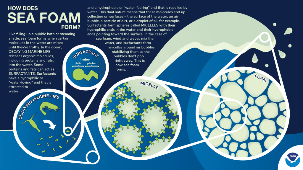
Figure 1-5. Formation of sea foam.
Source: NOAA (2024) Image credit: Kaleigh Ballantine/NOAA Office of Education
Although the primary source of surfactants in the ocean is the decay of dead algae and phytoplankton (particularly from “blooms”), PFAS are surfactants that can enhance foam formation, but are not required to be present. When the algae/phytoplankton die off-shore, they release large amounts of decaying matter, which can wash toward the shore, providing the surfactants necessary to form micelles. Foam forms as this organic matter is churned up by the surf and air is entrained below the ocean surface as in the first phase of aerosolization (NOAA 2024). This foam can be quite stable, in contrast to foam formed in nonsaline rivers, which generally exists for minutes to hours before collapsing back into the water column (see Section 16.5). The stability and nuisance factor of the ocean foam can be seen in this video: https://www.youtube.com/watch?v=rZM6SrFlxn0.
As with aerosolization, the entrained air bubbles scavenge PFAS, organic matter, and salts. During the collection of the stabilized bubbles and micelles, these scavenged materials are included in the formed ocean foam. The PFAS will be similarly enriched in the foam as it is in the SSA during aerosolization. This foam can remain near the shore, move onto the shore (as seen in the referenced video), or move out to sea. Over time, the foam will collapse, releasing SSA and some of the content of the bubbles back into the ocean water as the bubbles burst or fall apart.
Like aerosolization, ocean foam can transport enriched concentrations of PFAS beyond the source area (ocean water) and provide another route of exposure from contact with the foam or release from the foam as bubbles release SSA into the atmosphere.
1.3.5.4 Bioaccumulation of PFAS in Marine Biota
Although there are many studies on the bioaccumulation of PFAS in fresh water (see Section 5.5), there are fewer studies on the bioaccumulation of PFAS in marine waters. Some recent studies have reported the bioaccumulation of PFAS in apex predators such as sharks off the coast of the New York Bight, as far afield as the Bahamas (Lee et al. 2024), and in the northwest Atlantic Ocean (Marciano et al. 2024). As with freshwater studies, these show that longer chain PFAS (> C10) were frequently detected above reporting limits and concentrations were higher in blood plasma than in muscle collected from the same organism. With PFAS precursors detected in sharks from New York Bight but not the Bahamas, Lee et al. (2024) speculated that this reflected the greater diversity of PFAS sources in a highly populated region.
Khan et al. (2023) provided a comprehensive review of the scientific literature for PFAS bioaccumulation in marine organisms, looking at data for PFAS in wild marine organisms (invertebrates, fish, reptiles, birds, and mammals) from research over the past two decades. The authors also evaluated PFAS data for plankton, surface water, and sediment. Their review found patterns of PFAS accumulation consistent with those of freshwater studies, such as preferential accumulation of shorter chain PFCAs in plankton and longer chain PFCAs in invertebrates, fish, birds, and mammals, and generally higher body burdens of PFCAs and PFSAs in higher trophic-level organisms, with the overall highest levels found in marine mammals.
Burkhard (2021) conducted an evaluation of PFAS bioconcentration factors (BCFs) and bioaccumulation factors (BAFs) reported in scientific literature. Although the data are fairly rich for carbonyl and sulfonyl PFAS, the data for phosphate, fluorotelomer, and ether classes are poor to nonexistent. As with other studies for PFAS, Burkhard (2021) found that PFAS concentrations were greatest in liver and lowest in muscle, with whole body concentrations in between. A comparison of freshwater to marine water BCFs and BAFs was limited by the lack of data for marine organisms.
In a later study, Burkhard and Votava (2023) assembled biota-sediment accumulation factors (BSAF) for PFAS in 17 different taxonomic classes, with one of the objectives being to find out whether there are differences between freshwater and brackish/marine species. These authors found that the highest BSAFs were for bony fish and annelid worms, whereas certain plants and bivalves had the lowest BSAFs. Although a larger dataset was available for BSAF (compared to BAFs), the results were variable, with few differences observed between freshwater and marine species. The authors highlighted the need for more paired sediment:biota data with which to derive BSAFs in the marine environment. SERDP is currently conducting research into the environmental factors that influence PFAS bioaccumulation in the marine food web, Project ER22-3359. More information can be found on the SERDP website https://serdp-estcp.mil.
Last, as discussed by Higgins et al. (2007), because PFAS have different affinities for organic carbon in sediment and tissue residues are controlled by active transport rather than lipid, the theory of equilibrium cannot be used to describe PFAS partitioning. Hence, where there are data available, it is recommended that PFAS BSAFs be expressed as kg-organic carbon/kg-ww rather than as kg-organic carbon/kg-lipid.
1.3.6 Effects of Suspended Sediment on Surface Water Sampling and Measurement of PFAS
This section provides information regarding the development of surface water sampling efforts for PFAS, including in water bodies with high suspended solids content. This information builds on various sections that should also be reviewed to properly use the information provided here:
- Surface Water Sampling and Analysis, Section 16.4
- Transfer of PFAS Between Groundwater, Surface Water, Pore Water and Sediment, Section 5.3.4
- Sampling and Analytical Methods, Section 11.1
- Surface Water Body Secondary Sources, Section 10.3.1.2
Several factors can affect the concentration of PFAS in surface water samples. This is due in large part to the fact that PFAS tend to sorb to suspended sediments. Concentrations of suspended sediments in surface water increase during stormwater runoff events due to higher sediment concentrations in runoff and mobilization of sediment from the river bottom due to increased flow velocity. As a result, the sample location, timing of collection, depth, sample type (for example, aqueous, bed sediment, and (or) suspended particulate matter), and sample analysis methods (dissolved, solid phase, or total) should be considered when designing a surface water sampling plan. Whether investigating impacts from an individual source area or impact(s) within a watershed, an investigator may need to sample during ambient (baseflow) and various storm conditions (before, during, or after peak flow) to properly understand the PFAS source(s), concentrations, mobility, and impact. Section 5.3.4.2, Section 6.4, Section 11.1.7.3, and Section 11.2.1.2., discuss the collection and analysis of stormwater runoff samples provides additional information not provided by sampling conducted during ambient conditions.
Because this section discusses considerations on the design of a sampling plan to measure PFAS in surface water, it is intended to augment other references that detail the collection of water quality data in general. For example, the US Geological Survey has produced a National Field Manual for the Collection of Water-Quality Data (USGS 2019). That reference, along with additional references found in Section 1.3.6.1, and Section 16.4, provide information and guidance to help in designing and conducting a sampling and analysis plan for the collection of water quality samples from surface water, including some with PFAS-specific sampling techniques and some with an emphasis on stormwater.
1.3.6.1 Surface Water Sampling During/After Stormwater Runoff Events
Samples collected during ambient (baseflow) conditions reflect PFAS impacts from various non-stormwater-related discharges (groundwater discharging to a surface water body, wastewater, excess landscape irrigation, aerial or windblown deposition)). However, various factors affect a surface water sample collected during rain events, making planning, collecting, and analyzing the results of the sampling more complex. For example, a dilution effect can occur if the waters that are flushed from upstream areas and subbasins during rainfall events contain lower PFAS concentrations compared to the areas of interest, thereby decreasing the measured PFAS concentrations downstream. Conversely, rainfall events can also increase PFAS and PFAS-sorbed particulates in surface water from PFAS source areas (such as biosolids application areas, AFFF sites, industrial areas) and the general urban environment. This occurs by mobilizing particles and bottom sediments on which PFAS are sorbed as well as solubilizing PFAS on surfaces (Borthakur, et al., 2021). Rainfall can also flush and deposit atmospheric PFAS on the ground, freeing it to be carried to storm drains and eventually surface water. Rainfall events can remove microplastics from the atmosphere and ground surfaces and deposit them into surface water where they act as suspended particulate matter (SPM) that provides additional surfaces for PFAS and other pollutant adsorption, see Section 2.2.2 of the ITRC Microplastics (MP-1) Document (ITRC 2023). Thus, sampling only ambient conditions may not provide a complete understanding of PFAS impacts on surface water. Because rainfall often varies spatially and temporally (amount, intensity, and timing) across large watersheds, each storm may produce varying amounts of runoff from upstream subbasins, some of which may contain sources of PFAS and others not. The amount and source(s) of PFAS measured by the sample would depend in large part on storm dynamics in the watershed upstream of the sample location.
The degree of mixing within a stream may also influence how much of the dissolved and particulate-sorbed PFAS is measured at the sample location. That is, the PFAS may or may not be well mixed with depth or across the width of the stream, a condition that also holds for ambient flow conditions affected by wastewater and contaminated groundwater discharges (see Section 1.3.6.3).
In addition, stormwater events are associated with increased flow and turbulence in surface waters, along with additional mass of PFAS and other surfactant-type materials in the surface water. These conditions can lead to the formation of PFAS-containing foam. This foam removes a portion of PFAS from the water column, at least temporarily, and acts as a transport mechanism and new source of PFAS downstream or to another location when transported by wind away from the surface water. This complicates the assessment of PFAS in the water body. These concepts are discussed in more detail in Section 16.5 and in Section 1.3.5.3.
To summarize, ambient (baseflow) sampling and stormflow sampling measure different aspects and components of PFAS in a watershed. Depending on the sampling objectives, any surface water sampling plan should consider whether to sample during ambient flow, during stormwater runoff conditions, or both, and should consider sample location, timing, depth, and type (aqueous, solid phase, or total).
1.3.6.2 PFAS Concentrations and Transport During Stormwater Runoff
Several studies, including those described in Section 5.3.4.2, have shown changes in surface water conditions during stormwater runoff events that influence dissolved and sorbed PFAS concentrations. Some of the results depend on site-specific conditions. The findings include the following:
- Short-chain PFAS (those with less than 7 carbon atoms) predominated in the aqueous-phase. Long-chain PFAS (those with 7 or more carbon atoms) predominated in the sorbed phase (Ahrens et al. 2010).
- During stormwater runoff events SPM contained significantly higher concentrations of PFAS than the sediments on the water body bed, showing that the increase was related to runoff from PFAS source areas more so than mobilization of sediment from the bed (Borthakur et al. 2021).
- SPM increased during stormwater runoff events (Borthakur, et al. 2021).
- SPM can be a sink, source, or transport vehicle of particle-bound substances such as PFAS, metals, and polychlorinated biphenyls (Gockener et al. 2022).
- Concentrations of PFAS on SPM originating from PFAS-impacted source areas can be much higher than found on SPM by equilibrium distribution (Section 5.4.3.2).
- Microplastics entering the water body increase during the stormwater runoff event and taper off as microplastics have been removed from paved and soil surfaces, as well as from the atmosphere (see ITRC 2023).
- “SPM-bound PFASs are positively correlated with transparent exopolymer particles (TEPs) content, providing evidence that TEPs may accumulate and concentrate more PFASs on the SPM” (Shiu et al. 2023).
- Surface waters where the predominant PFAS sources are from wastewater discharges and similar point sources tend to have highest PFAS concentrations during dry periods when stormwater runoff is low. Conversely, when the dominant PFAS sources are nonpoint sources (for example, biosolids application areas), the peak concentrations are during periods of stormwater runoff due to mobilization of PFAS from the source areas and conveyance to the surface water body by stormwater (Carneiro et al. 2025).
In addition to the studies above, SERDP-ESTCP has several projects to evaluate PFAS in stormwater, particularly at military facilities. These projects primarily look at treatment technologies for removing PFAS from stormwater runoff. More information can be found on their website https://serdp-estcp.mil.
1.3.6.3 Hypothetical Scenario to Illustrate Surface Water Sampling
The following discussion provides a hypothetical scenario to illustrate key considerations for sampling of surface water and is based on the information presented in the preceding sections. In addition, information is included for high-turbidity samples.
Figure 1-6 is a conceptualized representation of surface water conditions and PFAS distributions in surface water. The upper portion of Figure 1-6 shows a cross-section in a water body during non-stormwater runoff events. PFAS are found throughout the water column with shorter chain PFAS more prevalent in the upper part of the water column and higher concentrations of longer chain PFAS sorbed to solids that are suspended in the water column and found in the river bottom sediments. River flows are not fluctuating significantly and PFAS molecules are in constant exchange, partitioning between the aqueous and solid states as mediated by the predominant sorption and desorption conditions. The riverbed is steadily being added to and moved slowly downstream.
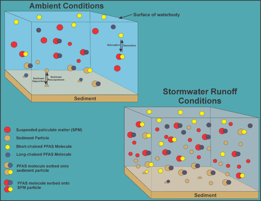
Figure 1-6. Water body conditions and conceptualized PFAS distributions.
Source: A. MacDonald, used with permission
The bottom right portion of Figure 1-6 shows the water column during a period of stormwater runoff. Total PFAS and SPM concentrations have increased. PFAS move between phases in response to differing mixtures and concentrations of PFAS, sorption to SPM and sediment, and concentration and makeup of SPM. Higher concentrations of SPM allow for additional sorption sites for PFAS and other pollutants. This sorption can potentially allow for increased PFAS transport downstream and deposit into the sediments of the riverbed. The system slowly reverts to ambient conditions as the storm subsides, and stormwater runoff ceases. Thus, depending on what questions are being addressed by collecting PFAS samples, the timing and location of sample collection must be carefully determined.
Factors Impacting When to Sample
PFAS concentrations and mass flux (concentration times the flow rate) in the aquatic system vary over time, during and following a storm. As discussed above, depending on the site and setting, storm flow that flushes otherwise PFAS-free subbasin(s) may dilute PFAS concentrations in downstream locations. Often though, during a stormwater runoff event, PFAS will increase in the receiving water, and be expected to eventually diminish as runoff ebbs and first-flush effects have mobilized available PFAS, with lesser PFAS amounts available for flushing as the storm continues.
If the goal is to evaluate the PFAS impacts associated with runoff from a single facility, there are numerous stormwater sampling guides established under National Pollutant Discharge Elimination System (NPDES) permitting programs by states and the federal government. The guidance provided in those documents was not developed with PFAS in mind, but the guides are applicable to PFAS. As examples, Oregon, Washington, and California, as well as USEPA, have developed such guides (WA Dept. of Ecology 2015; CA Water Boards 2001; USEPA 2021). These guides provide information on selecting locations, storm events to be targeted, and timing to obtain samples during the first-flush of stormwater runoff.
Sample timing in a larger target area such as an entire watershed or urban area is more difficult to establish, as there may be several PFAS source areas at varying distances from the water body being evaluated. Peak runoff from these areas may arrive at different times depending on local rainfall intensity, slope, and land cover. Determining the appropriate timing of sample collection can be difficult, so high frequency sample collection, collection of time-weighted composite samples, or using integrated samplers may be preferred to single grab samples to reduce the potential of missing high or low concentrations (Beisner et al. 2024). Single grab samples can augment the data collected by these other compositing/integrating sample methods.
Factors Impacting Where to Sample
The choice of sample locations depends on the objectives of the sampling. Do the objectives include looking for peak concentrations, average concentrations at a point in time, average concentrations over an extended period of time, concentrations that may impact benthic organisms or organisms residing in the water column or both, impacts associated with a particular site, impacts associated with an entire watershed, a need to provide information for selection and monitoring of PFAS treatment/mitigation measures, or any combination of these and other potential objectives? The degree of mixing within a water body will also affect the selection of sample locations. Below is an example that highlights sample location considerations and the above components for consideration. It uses concepts, designs, and nonspecific results from a study conducted on surface water impacts as part of an NPDES permit. The example does not specifically represent the location and specifics of that project.
Example of Where to Sample
Figure 1-7 shows an urban area with two major rivers, one tributary to the other. The river coming from the right is the dominant of the two and has received discharges from a vast expanse of farmland upgradient of the urban area. The river coming in from the left originated in the mountains and has received drainage predominantly from the mountains and part of the surrounding urban area. A significant amount of rainfall has occurred providing sufficient runoff meeting the criteria for collection of samples for evaluating impacts from stormwater runoff. Note the darker color of the river receiving runoff from farmland compared to the river receiving only mountain and urban runoff. This indicates a greater turbidity (increased SPM) from the farmland river along with a greater potential for PFAS associated with biosolids application. There are no known significant industrial sources of PFAS in the surrounding urban area. he objective of a proposed study is to determine the impact on the dominant river from the urban area.
Where, and from what depth should the samples be collected?
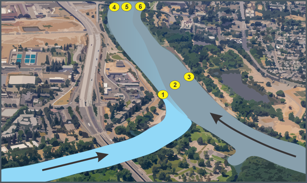
Figure 1-7. Example urban area with two major rivers.
Source: A. MacDonald, used with permission.
Discussion of sampling locations and depths
Because the goal is to determine impacts from the urban area, samples are needed just upstream of the first urban stormwater discharge points to the river to determine ambient concentrations. “Ambient” in this context means the river already impacted by the farmland, but not yet impacted by the study area. Those would be found upstream of points 1, 2, and 3, off the figure to the right. These samples would provide information for comparison to water quality standards and be used to determine the increase or decrease in PFAS concentration due to discharges from the urban area. Samples would also be needed at a downstream point in the river where there are no more urban stormwater runoff discharge points contributing to the river. This would be found some distance past the top of the figure. To determine which individual areas are contributing PFAS, point discharges of stormwater within the study area should be sampled. These sampling points would represent the discharge from the diffuse PFAS source areas in the watershed served by the discharge point.
If samples were to be collected at points labeled 1, 2, or 3 on the figure, the results could be misleading. Sampling at only location 1 would be representative mostly of the water entering from the river to the left. Sampling only location 2 would be representative of some sort of mixture of the two rivers. Sampling only location 3 would be representative only of the main river. The color of the receiving water provides a clue to the mixtures. One could sample all three locations and use the average of the three to represent the average concentrations across the cross-section of the river. However, this would likely not provide sufficient information for the study if there are additional urban inputs downstream. The same logic can be used for locations 4, 5, and 6. Ideally, the sampling is conducted even farther downstream, past all the urban discharge inputs and prior to other stormwater discharge inputs. If the downstream sample location occurs following a significant bend in the river that allows the river to mix across the entire cross-section, then representative samples can be gathered from several locations downstream of the bend. The concentrations could then be averaged if river velocity and depth of the river measurements are obtained at both the ambient and downstream locations. If that is not the case, then samples should be considered at several locations across the width of the river and at several depths at each location to account for some vertical stratification of SPM, resuspension of bed sediments, and potential reduced vertical mixing of urban runoff inputs.
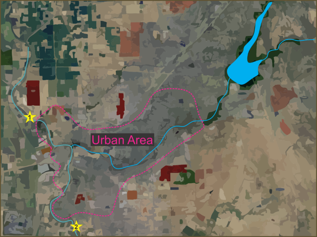
Figure 1-8. Example area with upstream and downstream locations identified.
Source: A. MacDonald, used with permission.
Figure 1-8 shows upstream sample location 1 and downstream location 2. Note location 2 is past the urban study area and downstream of a nearly 90-degree turn in the river, allowing for mixing across the river. Site-specific configuration of the river, and wastewater and stormwater discharge locations, will drive locations for sampling.
Because PFAS, if present, tends to be found throughout the water column, with a preference for some accumulation at the air-water interface (AWI), samples should be collected at several depths at a given location. The top sample would be at the AWI to include that accumulation site. The deepest sample would be near the river bottom to measure the higher turbidity that may be found there during higher river velocities mobilizing sediment. Additional samples between those two could be collected if needed, depending upon the depth of the receiving water and objectives of the sampling.
As mentioned above, there are many federal- and state-published guidelines on conducting sampling, including sampling to assess impacts of stormwater runoff. These should be consulted prior to developing a site-specific sampling and analysis plan.
Analytical Considerations with High Turbidity Samples
As described above, samples collected from stormwater and stormwater-impacted water bodies will have an increased solids content providing additional particles that can sorb PFAS and other pollutants. The analysis of high solids–containing samples (high turbidity samples) poses some additional complexity. This must be kept in mind and the objectives of the sampling must be discussed with the laboratory analyzing the samples so the analysis can provide the information needed to address those objectives. Section 11.2.1.2 includes information about preparing aqueous samples with particulates and suspended solids.
1.3.7 Source ID, Differentiation, and Forensics
This section supplements the material described in Section 10.5 and highlights key forensic concepts tailored to PFAS site characterization. Environmental forensics is a multidisciplinary field that integrates chemistry, environmental science, historical research, and data analytics to identify contaminant sources. Although many techniques used for legacy contaminants (for example, polychlorinated biphenyls, polyaromatic hydrocarbons, and dioxins) are also applicable to PFAS (Plumb 2004; Johnson et al. 2015; Cejas and Barrick 2020; Bock et al. 2021), PFAS present distinct challenges that require tailored interpretation strategies (Dorrance, Kellogg, and Love 2017; Morrison 2000; Morrison and Murphy 2006; Mudge 2008; Murphy and Morrison 2015; Sullivan et al. 2001; Wang and Stout 2006).
1.3.7.1 Lines of evidence
Unlike many legacy contaminants, PFAS forensic evaluations must account for precursor transformation, differential partitioning, and complex transport behavior that can alter chemical fingerprints over time (see Section 1.3.3, Section 1.3.4, Section 4, and Section 5). These processes can mimic or obscure source contributions if not properly considered.
Despite these challenges, several lines of evidence can support reliable source identification, including:
- unique compound ratios and isomer distributions reflective of specific manufacturing processes
- indicator PFAS associated with particular industries or waste streams
- distinct spatial trends influenced by differential sorption and migration
- precursor transformation signatures detectable via advanced analyses
- use of non-targeted analysis and suspect screening techniques to expand the analytical window and reveal compound classes unique to specific sources
The accuracy of forensic interpretations depends on integrating analytical results with contextual data, including site history, use patterns, and fate-and-transport mechanisms. When interpreted holistically, forensic approaches can offer critical insights into source apportionment and plume evolution.
1.3.7.2 Historical Research
Several studies have shown that many sites are impacted by multiple PFAS sources ( Anderson et al. 2016; Sun et al. 2016; Guelfo and Adamson 2018; Brusseau et al. 2020). This is particularly important in urban or industrialized areas. PFAS do not occur naturally but are found throughout the globe, including in remote areas (Herzke et al. 2023; Muir et al. 2019; Washington et al. 2019). Regional anthropogenic background levels reflecting nonpoint sources are present globally and can represent a significant fraction of the PFAS at a site. These ambient PFAS levels vary regionally and are often elevated in urban areas when compared to rural environments and remote locations (Section 6). In addition to identifying anthropogenic background, plausible PFAS-associated point sources in the vicinity of the investigation area should be identified and investigated.
Central to any source investigation is the evaluation of who or what may be wholly or partially responsible for site contamination based on when, how, and how much was contributed by each potentially responsible party (Sullivan et al. 2001). The answers to these questions almost always require an understanding of site history to develop information regarding:
- identification of possible local sources and site-specific anthropogenic background
- product usage history, accidental spills, or emergency response releases, environmental violations, waste handling, emission pathways and amounts
- plausible discharge pathways, such as aerial deposition, groundwater and surface water flow, soil disturbances and relocation
Numerous resources describe in more detail best practices for conducting historical research (Petrisor 2014; Sullivan et al. 2001; Murphy and Morrison 2015; Morrison 1999). The collected information should be interpreted in the context of the history of PFAS manufacture and use (Section 2). Note that historically, PFAS were often not included on material data sheets, therefore making it more challenging to determine whether historically used chemical formulations contain PFAS. As part of these investigations, surrogate non-PFAS markers of site wastes, discharge pathways, and transport pathways should be leveraged where appropriate.
1.3.7.3 Data Collection
Targeted sampling should follow historical research to test source hypotheses and characterize PFAS fingerprints (see Section 10 for field investigation strategies). This section highlights how analytical method selection can support forensic differentiation (see Section 11.2 for analytical methods for PFAS).
The diversity of PFAS formulations often necessitates looking beyond standard targeted methods. Although USEPA Method 1633A (2024) quantifies 40 PFAS, this may not fully capture site-specific profiles, especially when distinguishing between AFFF and non-AFFF sources.
To increase forensic resolution, high-resolution mass spectrometry techniques such as suspect screening and non-targeted analysis can detect a broader range of compounds and isomers, including precursors and source-specific chemistries (Glüge et al. 2020; Dasu et al. 2022). These approaches improve the statistical power and granularity of source attribution analyses (Strynar et al. 2023; Transport Research, Board NASEM 2023).
1.3.7.4 Preliminary Data Evaluation
Prior to applying advanced visualization techniques or multivariate data analytics methods, preliminary evaluation of the data quality is necessary. The integrity of forensic conclusions depends on understanding and addressing several common data issues:
- Censored values (below the detection limit): Nondetects should be reviewed in the context of detection and reporting limits, which may vary across samples or compounds. Decisions on data treatment (for example, substitution, statistical imputation) should align with data quality objectives (USEPA 2006; Helsel 2010).
- Approximate values (above but near the detection limit): Detected concentrations below the reporting limit may introduce uncertainty. Their influence on PFAS fingerprints should be evaluated, especially if they constitute a large portion of a profile.
- Extreme values (potential anomalies/outliers): Outliers may reflect analytical error or real, high-concentration releases. Graphical and statistical tools can help determine if such values distort the interpretation or reflect site-specific events (Helsel et al. 2020).
- Missing values (data gaps due to variable analytical methods): Variability in analytical methods over time (for example, USEPA Methods 537, 537.1, 1633A; see Section 11.2.1 for more information about quantitative analytical techniques) can result in inconsistent compound lists. This may necessitate focusing multivariate analyses on a common subset of analyte, or the use of methods that accommodate missing data.
Early-stage data screening helps guide appropriate methods for fingerprinting, visualization, and multivariate evaluation. These steps support robust forensic interpretation by ensuring that statistical outputs reflect meaningful environmental trends rather than analytical artifacts.
1.3.7.5 Data Visualization
Typical site characterization visualization methods such as groundwater iso-concentration plume maps, hydrogeologic cross-sections or fence diagrams, and 3-D CSMs may be used to depict the horizontal and vertical extent of PFAS. Other visualization methods that depict the relative or absolute abundances of the various PFAS include:
- Bar charts: Side-by-side comparison of multiple PFAS (the bars), with bar height relating to relative or absolute abundance (Figure 1-9). Many constituents can be shown on a bar chart, with the overall pattern of the bars forming a sample’s profile.
- Pie charts: Circular graphic (Figure 1-10) with compounds represented as adjacent quadrants and area proportional to relative abundance. Pie charts are readily displayed on maps.
- Radar plots: Circular graphic with concentrations displayed on individual axes, with increasing values away from the center (Figure 1-11). Unique fingerprints often form distinct shapes on a radar plot.
- Ternary plots: Triangular plots that depict the relative proportions of three PFAS in a mixture (Figure 1-12). These plots are commonly employed in soil science to differentiate soil types consisting of differing proportions of grain sizes, and in chemistry to differentiate chemical mixtures, among other applications.
- Scatter plots: Comparison of chemicals on rectangular (Cartesian) axes, to assess correlation, groups, or other trends.
- Family tree–style 3-D bar charts (Gamlin et al. 2024).
Bar, pie, and radar charts may be further enhanced by organizing PFAS by functional group, and sorting by physicochemical properties (chain length). Organizing the data in this way can assist with the interpretation of perfluoroalkyl carboxylic acid (PFCA) versus PFSA content and shed light on potential fate-and-transport signatures (that is, differential presence of shorter chain compounds). Section 10.5.1.3 includes examples of visual representations of data. Additional figures are included here.
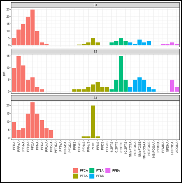
Figure 1-9. Comparison of PFAS signatures in samples S1, S2, and S3 using bar graphs. The concentration of each PFAS is shown on the y-axis, with the y-axis for each sample separately to maximize the plot area.
Figure source: Provided by Michael Bock, PhD. Used with permission.
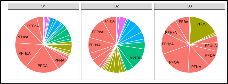
Figure 1-10. Comparison of PFAS signatures in samples S1, S2, and S3 using pie charts. The concentration of each PFAS has been divided by the sum of all measured PFAS to represent the relative abundance of PFAS in each sample.
Source: Provided by Michael Bock, PhD. Used with permission.
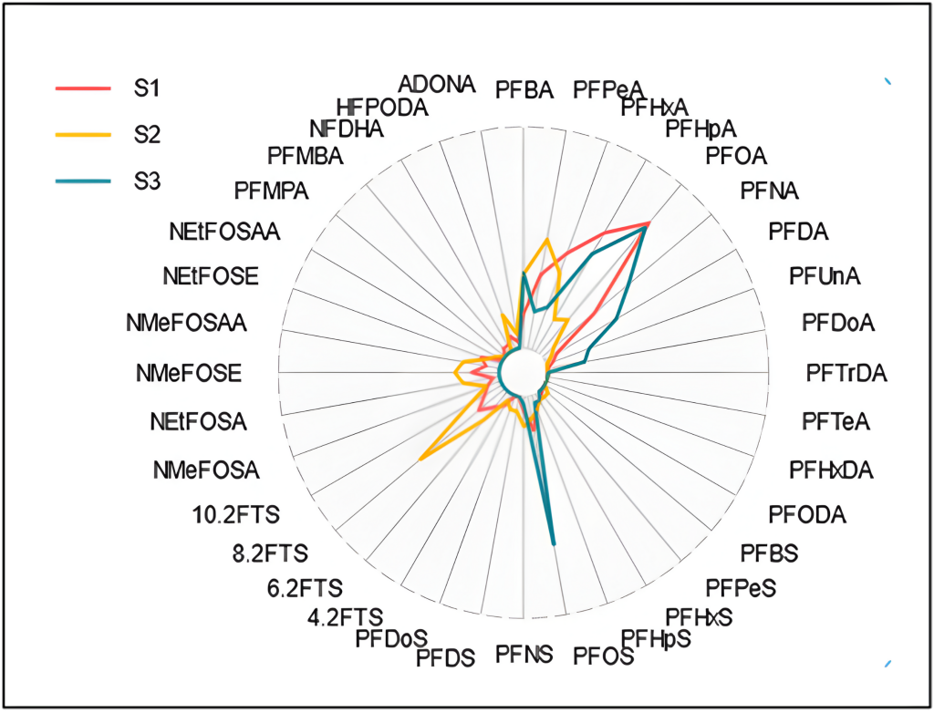
Figure 1-11. Comparison of PFAS signatures in samples S1, S2, and S3 using radar plots. The concentration of each PFAS has been divided by the sum of all measured PFAS to represent the relative abundance of PFAS in each sample.
Source: Provided by Michael Bock, PhD. Used with permission.

Figure 1-12. Comparison of PFAS signatures in samples S1, S2, and S3 using a ternary plot. The ratios of PFBA, PFOA, and PFOS in each sample are plotted.
Source: Provided by Michael Bock, PhD. Used with permission.
In some applications of PFAS forensics, it may be beneficial to show similarities or differences between samples using either the concentrations or relative abundances of one or more PFAS ratios. Double ratio plots (Figure 1-13) are a common tool in polycyclic aromatic hydrocarbon forensics (Sauer and Uhler 1994; Douglas et al. 1996; McCarthy et al. 2000), where ratios of one or more constituents are shown on the axes of a scatter plot. Double ratio plots greatly enhance the power to differentiate between samples and sources and have been applied to PFAS forensics.

Figure 1-13. Comparison of PFAS signatures in samples S1, S2, and S3 using double ratio plots. The ratios of PFBA/PFNA and PFOA/PFOS in each sample are plotted.
Source: Provided by Michael Bock, PhD. Used with permission.
Raup et al. (2024) (see Section 15.1.4) used pie charts to depict fingerprint changes between surface water and overburden and bedrock groundwater, with potential contributions from septic systems. For this study, six PFAS were selected based on drinking water criteria, but a larger analyte list could potentially reveal more nuances in the chemical signatures. Tracers, such as artificial sweeteners and nitrogen species, were used alongside other lines of evidence (such as nearby wastewater treatment plant sample signatures) to support the notion of septic or other source contributions, or both. Ratios between PFAS concentrations and total PFAS clarified fingerprints within and between sampling areas, as well as potential source types. Low standard deviations calculated for many ratios indicated general geographic homogeneity of the signatures. Means and standard deviations served as statistical indicators for anomalous samples that could represent potential sources and further characterization targets. Additional case study examples are discussed in Section 15.1.
Gamlin et al. (2024) recently introduced a new method to visualize PFAS sample profiles (Figure 1-14). The method helps in identifying and interpreting patterns by organizing data by PFAS class, carbon number, and oxidation state. The concentrations or proportions are shown using 3-D bar plots. This framework can incorporate any analyte list, allowing it to evolve with advancements in analytical capabilities and scientific understanding. A 3-D modification of the Gamlin plot permits depiction of concentration levels as well.

Figure 1-14. Comparison of PFAS signatures in two samples from Gamlin et al. (2024).
Source: Open Access. Gamlin et al. (2024). https://creativecommons.org/licenses/by/4.0/
Most plots discussed here share a common disadvantage that only a few samples may be shown at a time, necessitating advanced (multivariate) methods that address the full chemical profile of many samples simultaneously.
1.3.7.6 Fingerprinting Calculations
Correlation coefficients and cosine-theta are two similarity indexes that are commonly used in a forensic evaluation to compare samples to each other and to sources (Davis 2002; Johnson et al. 2006). They have both been applied to PFAS forensics (Rose et al. 2024). These methods are adaptable to various PFAS sources and can be used to refine CSMs for better risk assessment and remediation. The correlation between two samples is calculated by ordering the PFAS in each sample before calculation. The resulting correlation coefficient provides an index of the similarity between these two samples. When calculated across many samples, the correlation matrix can be used to identify similarities. As with correlation metrics, cosine-theta provides a relative index of pattern or signature similarity of PFAS from samples, wells, or sources. It is also used to identify PFAS families in various cluster analysis approaches. No threshold value indicates a match (Johnson et al. 2006), but rather the determination of the strength of any match is based on the professional judgment of the statistician and the reader.
Figure 1-15 shows a Pearson’s Correlation matrix and cosine-theta matrix for the sample profiles depicted in Figures 1-9 through 1-13. In the two matrix plots, higher values (illustrated with the color ramp from purple, low values, to yellow, high values) indicate a higher degree of similarity between the samples, with samples S1 and S3 being the most similar (lighter orange), S1 and S2 the next most similar (orange and pink), and S2 and S3 the least similar (darker pink and purple). The results demonstrate that these indexes provide a relative indication of similarity. It is up to the statistician to assess the importance of the specific values of these indexes. It is up to the statistician to assess the importance of the specific values of these indexes.
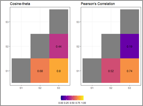
Figure 1-15. Comparison of PFAS profiles in three samples using cosine-theta and Pearson’s correlation coefficients as a matrix. These are the same PFAS profiles depicted in Figures 1-9, 1-10, 1-11, 1-12 and 1-13.
Source: Provided by Michael Bock, PhD. Used with permission.
Correlation coefficients, such as Pearson, Spearman, or Kendall, can detect monotonic positive or negative relationships between columns of data, such as assessing the similarity of concentration trends between individual PFAS, between PFAS and other environmental chemicals (co-contaminants), or between PFAS and potential site-specific explanatory variables (distance to a source). For example, Pearson’s correlation (r) compares observations, means, and standard deviations of two data columns, such that higher values near 1.0 indicate a strong, positive linear correlation, values near -1.0 indicate a strong, negative linear correlation, and values near 0.0 indicate no correlation (Helsel et al. 2020). Strong positive or negative correlations may indicate that spatially and temporally, individual PFAS align with specific spatial site features or other contaminants (or their absence). This type of assessment may be useful for assisting the interpretation of sources and subsurface processes.
Cosine-theta similarity is a traditional fingerprinting metric that geometrically represents the vector correlation between two data rows/samples (Nagai et al. 2019). The dot product produces a measure of alignment between chemical signatures, yielding a value of 1.0 for perfectly matching rows, and 0.0 for rows that do not match at all. This calculation is helpful for comparing a sample of unknown origin with a known or suspected chemistry source profile, to check for a positive match.
Together, these methods are adaptable to various PFAS sources and can be used to refine CSMs for better risk assessment and remediation. They support and are augmented by advanced analytics calculations that may more fully describe column-wise correlation (dimensionality reduction/regression) or row-wise similarity (clustering/classification).
1.3.7.7 PFAS Isomers
The PFAS analytical results described and visualized above combine the results for the various isomers into a single value (see Section 11.3.5 and Section 11.4.2 for more information about analyses of linear and branched isomers). As described in Section 3.5, PFAS such as PFOA can exist as a variety of isomers that have the same chemical formula, and the relative abundance of different isomers can be diagnostic of the original source. The ratio of branched to linear isomers is typically used to differentiate between PFAS produced using the electrochemical fluorination (ECF) process versus the telomerization process. For example, ammonium perfluorooctanoate (APFO)/PFOA was produced between 1947 and 2002 through ECF. Post-2002, virtually all PFOA was produced by telomerization. The ECF process would be expected to produce 70%–80% linear PFOA isomers and 20%–30% branched PFOA isomers while the telomerization process would produce 100% linear isomers (Buck et al. 2011). If investigators suspect multiple sources may be present in a PFAS plume, quantification of branched isomers may be an important line of evidence to show that an additional source exists or begin to identify its location. However, postrelease fate-and-transport processes may affect the distribution of the different isomers (see Section 5; Schulz, Silva, and Klaper 2020), potentially masking the isomeric composition of the original source material, so care must be taken when interpreting PFAS isomer data as a line of evidence in a forensic evaluation.
1.3.7.8 Data Gaps
Following the initial field investigation and data visualization, data gaps may become apparent that warrant additional sampling. For example, if sampled locations do not reflect known historical site processes or contaminant migration pathways, further sampling of source areas may be required. Inspection of concentration maps or time-series charts may also reveal potential but incomplete trends that would benefit from further characterization. Finally, additional quality assurance/quality control (QA/QC) samples may be needed to demonstrate exceptionally high or low levels of PFAS in a given area or vertical zone.
1.3.7.9 Advanced Data Analysis
At its core PFAS forensics is largely derived from, and benefits greatly from, the lessons that have been learned from the rich history of chemical forensic methods and applications. Multivariate methods have been applied to investigate sources of PFAS across the globe in a variety of matrixes, from serum in the Faroe Islands (Hu et al. 2018), to surface water in the United States (Zhang et al. 2016), and sediment in China (Pan et al. 2014). Multivariate methods are broadly categorized as self-training (unlabeled data) or predictive (labeled data). There is an acknowledgment in the forensics literature that many of these legacy methods generally fit under the umbrella of machine learning.
Self-training methods, which derive patterns without explicitly predefined labels, have been used for fingerprinting other chemical mixtures for decades. Recent years have seen an increased focus on predictive methods, where the data are linked to one or more columns of labels. Both approaches are described in more detail below in the Self-training Methods and Predictive methods sections.
Self-training Methods
Self-training methods are unique for forensics investigations, in that the algorithm is not provided a starting point with labels for the source profiles but rather uses the data itself to develop the model. PFAS signatures are inherently multivariate in that they comprise mixtures of multiple compounds. Often, site-specific chemistry data lack well-characterized source sampling records or clear, representative sampling locations for ambient levels. This makes it difficult to distinguish a range of different source profiles from each other or from fate-and-transport signatures, or to separate nonpoint ambient levels from nonpoint impacts. Certain algorithms, such as dimensionality reduction and clustering, are self-training in that they have been used to derive source (and other) signatures and latent (not explicitly measured) structure in the data.
Dimensionality Reduction
The objective of dimensionality reduction is to capture the essence of many data columns (that is, analytes) and express it with fewer columns (that is, relative source contributions). This operationally distills the data structure into a more focused format for an analyst to understand sources and their contributions. Dimensionality reduction can be performed in multiple ways, each with a different objective.
Principal Components Analysis
Principal components analysis (PCA) was first proposed by Karl Pearson in 1901 (Pearson 1901). It fits a series of orthogonal lines (the principal components) through a data cloud to preserve its variance. Often, PCA is performed using singular value decomposition (Joliffe and Cadima 2016), which resolves the data table into scores (representative of the data rows) and loadings (representative of the data columns). Visualized together on the same graphic, scores and loadings form a biplot, permitting the user to assess the relative effect of each analyte loading on each sample (score), as well as the overall configuration of the data cloud (Figure 1-16). Figure 1-16, Figure 1-17 and Figure 1-18 use the same data. Fiedler et al. (2022) used PCA to identify correlations of three PFAS in multiple media and their trends in 266 samples from 26 developing countries, finding generally higher levels in biotic solid media from the Caribbean and Latin America. Li et al. (2022) likewise used PCA to differentiate trends in Florida surface water from four regional sampling locations, and in tap water from three regional locations. Antell et al. (2024) incorporated total oxidizable precursor (TOP) assay data into PCA to differentiate trends and patterns, separating multiple potential PFAS sources, including AFFF, wastewater treatment plants, and landfills. In each publication referenced above, biplots were used to draw visual conclusions regarding the separation or overlap of different groups, and assess trends in the data cloud pertaining to different PFAS chemicals, separating multiple potential PFAS sources, including AFFF, wastewater treatment plants, and landfills. In each publication referenced above, biplots were used to draw visual conclusions regarding the separation or overlap of different groups, and assess trends in the data cloud pertaining to different PFAS.
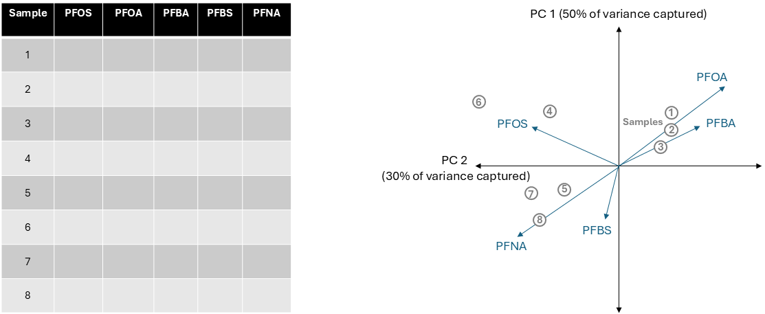
Figure 1-16. Example of a PCA biplot. Data columns (PFAS) are displayed as arrows and mathematically related to rows (samples) that are displayed as points. Sample position along the direction of an arrow indicates more of a specific compound, and proximity to other samples indicates chemical similarity.
Source: S. Sorsby, WSP. Used with permission.
Receptor Models
Similar to PCA, receptor models use a variety of similar methods collectively called factor analysis to likewise resolve a chemistry data table into scores and loadings. However, forensic use of factor analysis typically does not require the loadings to be mathematically orthogonal, and instead are permitted to align obliquely with unique signatures in the data (that is, potential sources or fate-and-transport patterns; (Figure 1-17). Depending on the method of preprocessing used, patterns derived by receptor models may approximate sourcelike compositions. As part of the receptor modeling process, the user must specify the number of unique signatures to derive, requiring site-specific knowledge to make a reasonable estimate. Capozzi et al. (2023) used positive matrix factorization to assess PFAS signatures related to a nearby landfill, and make inferences about precursor depletion in the subsurface. Wang et al. (2022) used a similar method—nonnegative matrix factorization—to identify groundwater PFAS signatures, including a signature dominated by short-chain compounds interpreted to represent the phaseout of legacy PFOS and PFOA. Rose et al. (2024) used polytopic vector analysis to assess the effects of variable seeding methods, sample size, and noise on factor analysis of synthetic PFAS datasets with literature-based source profiles, with better results for datasets of 25 or more samples and specific automated seeding methods.
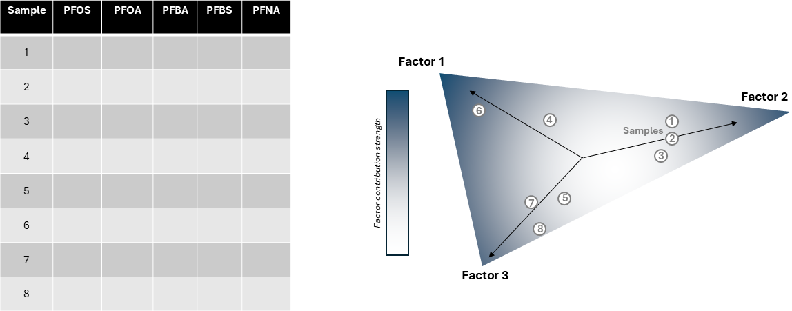
Figure 1-17. Conceptual schematic of a receptor model/factor analysis. Data columns are combined into primary chemical profiles and represented as directions in the data, pointing to corners of the data cloud (fingerprints). Sample (point) proximity to a corner is proportional to the strength of the corresponding signature.
Source: S. Sorsby, WSP. Used with permission.
Manifold Learning
A newer class of dimensionality reduction methods, known as manifold learning, has emerged. Uniform Manifold Approximation and Projection (UMAP) is an example of manifold learning whereby the chemical similarity of samples (that is, the manifold) considering all data columns is preserved in fewer columns. Unlike PCA and receptor models, manifold learning methods are nonlinear and can fit to curved regions of the data cloud. Antell et al. (2024) used UMAP to strengthen differentiation of source signatures using TOP assay data, including different AFFF formulations.
Dimensionality Reduction Method Selection
Several concepts should be kept in mind when selecting a dimensionality reduction method. Because PCA identifies orthogonal directions in the data, it is good at summarizing the data cloud in a way that is visualized in 2-D or 3-D with Cartesian coordinates (that is, standard scatter plot axes). However, the principal components themselves do not describe source signatures unless the sources themselves align with the axes. Receptor models resolve oblique angles in the data that may more accurately represent source signatures. However, additional lines of evidence are necessary to determine the number of factors to use. Nonlinear methods such as t-distributed stochastic neighbor embedding (t-SNE) and UMAP identify potentially nonlinear structure in the data and warp the manifold to fewer dimensions for easy visualization. The principal advantage of these methods over PCA is that all the variability is expressed in two axes of one plot while with PCA only a fraction is expressed. The disadvantage is that the reduced dimensions are still subject to complex sample relationships (that is, are modeled with network graphs), and groups and trends must be interpreted carefully by an experienced analyst. Most manifold learning methods do not capture the relationship between columns (analytes) and rows (samples).
Clustering
Unlike dimensionality reduction methods that identify numeric trends in the data, clustering methods identify categorical groups. Some methods, such as K-means, identify optimal partitions between discrete bins of similar data points. Others, such as Gaussian mixture modeling (GMM), rely on underlying statistical properties to resolve potentially overlapping groups. As with receptor models, clustering methods require the user to estimate the number of signals present in the data. If the user-specified number of clusters is more than the actual data structure accommodates, contiguous samples may be artificially separated into different signatures. Inspection of resolved clusters is needed to verify the outputs of partitioning methods.
Partitioning Methods
Partitioning-based cluster methods are helpful for quickly identifying groups that are clearly separated, by relating sample chemistries into similar groups (Figure 1-18). Zeng et al. (2024) used K-means to derive clearly distinct signatures differentiating various industrial, agricultural, and domestic sources of PFAS to the Pearl River Basin. Zhang et al. (2016) used hierarchical clustering to identify major sources of PFAS contamination in diverse watersheds in the northeastern United States. PCA and hierarchical clustering identified three distinct groupings of PFAS, showing different mixtures of compounds at various sites. Clustering-derived signatures were interpreted to relate to contemporary point sources such as airports and textile mills, waste-sector sources, and metal-plating operations. Ogunbiyi et al. (2024) studied the distribution of PFAS in surface and bottom water from the inshore and offshore areas in the Biscayne Bay area (Miami, FL) using the K-means clustering algorithm.
Results included three distinct clusters, each interpreted to represent different sources or levels of PFAS contamination associated with industrial discharge, urban runoff, or atmospheric deposition/agricultural runoff. The geographical mapping of these clusters revealed that industrial discharge was more prevalent in areas close to manufacturing sites, while urban runoff was dominant in densely populated regions, key supporting lines in a forensic evaluation.
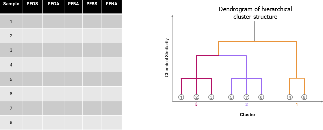
Figure 1-18. Conceptual schematic of hierarchical clustering analysis. Samples (“leaves”) are terminal nodes in a treelike “dendrogram” that catalogs chemical similarity by joining them together with successive “branches,” until all are related. “Cutting the tree” at a certain level returns cluster groupings at that level of similarity.
Source: S. Sorsby, WSP. Used with permission.
Probability-based Methods
Probabilistic clustering methods, such as GMM, fit potentially overlapping statistical distributions to the data to resolve groups. Due to the additional information provided by using prespecified statistical distributions, goodness-of-fit metrics such as Bayesian information criterion may be computed to assist with the selection of the number of clusters. GMM was proposed for use in characterizing site-specific metals background levels in soil (USEPA 2019). Anderson and Modiri (2024) later used a large dataset comprising thousands of surface soil samples from Air Force bases, representing both anthropogenic background and AFFF-impacted soils. GMMs were applied to log-transformed PFOS concentrations to model the distribution of PFOS in these samples. Various methods were employed to handle nondetects (approximately 8% of the data). Multiple GMMs were fitted, each with different numbers of components to capture the distribution of PFOS concentrations. Goodness-of-fit measures, such as the Bayesian information criterion and Akaike information criterion, were used to evaluate the models. These diagnostics were interpreted to support the existence of two clusters, establishing a general ambient range of potential nonpoint-source levels for PFAS, and distinguishing them from AFFF-impacted soils.
Clustering Method Selection
Several considerations may assist users in the selection of a clustering method. Theoretical support for the presence of underlying distributions would promote the use of statistical model-based methods such as GMM. These methods are also amenable to resolving overlapping clusters. Partitioning-based methods may be useful in situations where clusters are more clearly resolved or do not adhere to a set of theoretical probability distributions, or both.
Predictive Methods
Some statistical models are called predictive, in that they mathematically link user-specified input variables to one or more categorical or continuous output variables. Unlike self-training methods discussed in the Self-training Methods section above, the user must specify the continuous target (in the case of regression) or a categorical target (in the case of classification). Due to the requirement of prespecified labels, careful problem framing is required. It is important to keep in mind that statistical models do not typically incorporate physical or chemical heuristics (as a fate-and-transport model would), and must be interpreted as a line of evidence alongside physical and chemical site conceptualizations.
Regression
Regression methods relate one or more input data columns (X) to one or more numeric output columns (Y). Due to the requirement of the output column(s) to be of numeric form, regression-based approaches to PFAS forensics in the literature have mostly focused on relating PFAS concentrations to other variables, to add contextual links for source identification and environmental occurrence. An approach of this nature is a more advanced form of correlation analysis, relating potentially many drivers, co-contaminants, or other explanatory features to one or more outputs (PFAS levels). As with a correlation analysis, regression may be helpful as one line of evidence to support the overall conclusions of forensic investigation but should be accompanied by other lines of evidence.
Linear regression is a long-standing example of this effort, where the relationship(s) between inputs and outputs are linked by slopes and an intercept. Hu et al. (2016) used multiple linear regression to relate a large dataset of US drinking water samples from the US EPA UCMR3 program to the abundance of source types (major industrial sites, military fire training sites, AFFF-certified airports, and wastewater treatment plants) in eight-digit hydrologic-unit code watersheds. The results indicate that the source sites in a given watershed correlated with higher PFAS concentrations of PFBS, PFHxS, PFHpA, PFOA, PFOS, and PFNA, potentially linking impacts to their corresponding source types and providing diagnostic indicators for sites within a given watershed.
Other regression models used in the environmental sciences include nonlinear tree-based models. Breitmeyer et al. (2023) correlated the sum of 33 target PFAS from 161 sampled streams to land-use features and potential sources via a conditional inference tree. They found that upstream urban developments were a primary driver of general increases in PFAS concentrations, with proximal water-pollution control and electronic-manufacturing facilities as key potential sources to surface water. As with Hu et al. (2016), regression formed the basis for linking specific source types to PFAS impacts in a forensic context.
DeLuca et al. (2023) used a random forest regression model to leverage geographic and industrial variables to predict the spatial distribution of summed PFAS in fish tissue due to a variety of sources in the Columbia River Basin of Washington State. Like other regression-based studies, the inclusion of a variety of potential sources in the analysis permitted forensic insight. Important drivers of PFAS in fish potentially included proximity to fire training facilities, metal coating facilities, paint facilities, and airports. The authors noted that cement manufacturing and glass production facilities were also scored as potentially significant drivers of PFAS contributions to surface water, although they were among the least represented industries in the dataset and should be interpreted carefully. The use of a “PFAS prospecting” regression model to support forensic inferences could hence support the identification of local sources or ambient levels of PFAS to environmental media and reveal potential data gaps in a source location analysis (undersampled/understudied pathways).
Classification
Classification methods relate one or more input variables to a categorical output. In environmental forensics, source types are a popular categorical association made during identification and allocation. Due to the relatively straightforward problem framing of relating source type labels to chemistry data, classification methods are more prolific in PFAS forensics literature. Prediction of source type based on chemistry data is useful as a screening tool to assist with characterizing impacts of unknown origin. As with other methods presented in this document, it is important to apply methods on a site-specific basis, or otherwise bring site-specific insight into a more generally trained model.
Kibbey et al. (2021) focused on distinguishing between AFFF and non-AFFF sources to groundwater PFAS impacts, using 12 different classification methods. Of the 12 methods, random forest and neural network classifiers were found to exhibit the highest accuracy (96.1% and 95.5%, respectively). The authors noted that PFAS with higher frequency of detection were generally more predictive features in the classifiers.
Kibbey et al. (2024) explored multiclass classification of PFAS sources, including AFFF, wastewater treatment plants, and landfills. The authors employed a tiered framework to identify chemical profiles from a variety of sources, and to recognize novel samples that differed from any sources in the training dataset. Blind prediction of site samples indicated reasonable predictive capability of the model. This study raises the important question of novel samples, which are different from all previously trained data classes, which must be considered when building a classification model.
Joseph et al. (2023) employed a supervised machine learning approach using support vector machines to classify PFAS sources. Support vector machines are particularly adept at handling high-dimensional data, which is common in PFAS analysis due to the large number of compounds and potential sources. The researchers used a kernel function to transform the data into a higher-dimensional space, making it easier to find a hyperplane that separates the classes. The study successfully identified distinct PFAS profiles for AFFF-impacted groundwater and landfill leachate, demonstrating the potential of support vector machines in environmental forensics.
Antell et al. (2024) created a predictive classifier that uses TOP assay data to predict source types. Sources included were AFFF sites, wastewater treatment plants, and landfills. A custom nearest-neighbor search algorithm was used to associate samples with source types. Preprocessing the data via principal components analysis improved the resolution of the classifier, with 88%–99% accuracy of the sources.
Predictive Method Selection
The choice between regression or classification methods varies depending on the study objective. When a numeric value is desired, regression methods may be used. Classification methods are suited for separating samples into different, user-specified groups.
To select a regression-based method, there are several considerations. Target (dependent) variables must be screened for extreme values, as these points may exert higher leverage during the fitting process and focus on less-representative structure in the data. Data transformations, such as logarithms or square roots, may assist in reducing the influence of extreme values deemed representative of site data. The relationships should also be assessed for nonlinearity. In the event of a nonlinear dataset, inclusion of feature interactions may make linear regression flexible enough to adequately fit the target, but must be assessed by an experienced practitioner. Nonlinear regression algorithms, like decision trees, may capture nonlinear structure. Care must be taken to not “overfit” the data (memorize the inputs without abstracting well), which may be alleviated by ensemble-based nonlinear regressors (for example, random forest or xgboost).
Classification methods likewise require a consideration of linearity. For classes that are visually separable by a straight line on a scatter plot, linear methods such as logistic regression or linear discriminant analysis may suffice. Nonlinear decision boundaries between classes may require a more flexible model, such as k-nearest neighbors or a decision tree. As with regression methods, ensemble models such as random forest or xgboost may achieve a balance of accuracy and generalizability (avoids overfitting), with sufficient tuning by an experienced user.
1.3.7.10 Model Validation
An often-overlooked aspect of many of the multivariate methods and models applied to PFAS forensics is validation. As with any statistical model, validation of the model should not be overlooked. Johnson et al. (2015), Gauthier and Hawley (2007), Ginevan (2007), and Bock et al. (2021) provided useful examples of model validation methods and examples of their use. Basic model validation techniques and tools include:
- comparison of the modeled versus the original chemical profiles, often in the form of bar plots
- plot of observed versus modeled, including the 1:1 best fit line
- goodness-of-fit statistics such as cosine-theta, r2, and mean squared error
- evaluation of the data for trends unrelated to the CSM, such as systematic differences between analytical laboratories, analytical methods, or samples collection methods
- rigorous evaluation of the CSM, hypotheses, and alternative hypotheses. For example, is a change in profiles attributable to:
- different sources.
- differential fate and transport.
- precursor transformation.
- comparison to source libraries
- comparison to potential anthropogenic background levels and profiles
PFAS mixtures are frequently impacted by nonpoint sources. These nonpoint sources are often classified as anthropogenic background, regional nonpoint sources, or baseline (see Section 10.2). The influence of potential anthropogenic background can be an important component of the results of a forensics evaluation. A discussion of methods to characterize anthropogenic background is beyond the scope of this section, but understanding how they can influence a forensic evaluation and how they are considered in the CSM should be determined prior to beginning the investigation.
1.3.8 Site Characterization Tools and Techniques
This section supplements the information in Section 10 on unique considerations for PFAS site characterization and provides practical guidance for conducting PFAS site characterization, including strategy, approach, tools, and techniques. Because of the unique properties and environmental behavior of PFAS, site characterization efforts at PFAS sites may require collecting different types of information compared to investigations for other types of contaminants. Some tools provide one line of evidence, while others may have the ability and data to support more than one. This approach to assembling the key elements of site characterization is supported by Section 11, which provides greater detail on sampling and analysis tools and techniques for specific data acquisition.
1.3.8.1 Investigation Approaches
Investigation approaches are typically based on project goals and site characteristics, including but not limited to site history, setting, watershed characteristics, number and types of sources, and potential receptors. Two approaches are discussed below: “outside in” and “inside out.” While each approach is described separately for simplicity, a combined or hybrid approach might be appropriate, depending on the characteristics of the site, regulatory program requirements, and other factors.
Outside-In Approach
The outside-in approach is generally based on a receptor-protection concept, whereby the extent of PFAS migration is identified first along with affected receptors, if any, distal to on-site PFAS sources. This would involve prioritizing the sampling of potential receptors (for example, supply wells, surface water bodies) and downgradient monitoring locations before source identification and pathway characterization. The investigation would then proceed back toward the site of interest and to on-site source locations. Though appropriate for proactive receptor protection, this approach may be confounded by commingled PFAS from other sources, especially in industrialized areas and where such facilities share a common surface water body to which PFAS discharge. An outside-in approach may be the only option when a PFAS plume has been identified without knowledge of the source.
Inside-Out Approach
This approach applies to the characterization of discrete sources of PFAS interior to a site and the investigation of potential migration pathways from those sources to delineation, receptors, or boundary conditions. Where such delineation is feasible, it will provide higher confidence in understanding overall impacts and long-term fate and transport concerns.
The inside-out approach is incremental and sequential, as follows:
- identify potential on-site sources of PFAS based on site history and use
- conduct targeted soil and groundwater sampling to confirm presence of PFAS associated with the release or application locations
- conduct broader lateral and vertical soil and groundwater sampling for PFAS to determine nature and extent from the source
- sample groundwater and surface water migration pathways until delineation, boundary condition, or receptor is encountered
- focus management measures on the source-pathway-receptor connection
This approach allows the investigator to isolate and proactively address PFAS occurrence emanating from a specific source and along migration pathways.
1.3.8.2 Surface Water Receptors
In many jurisdictions, surface water criteria are close to analytical detection limits due to concerns about bioaccumulation of PFAS and emerging human health criteria (for example, reference doses [RfDs]) related to surface water uses (see Section 16 and the Environmental Media Values Table). Surface water receptors may be a sink for PFAS released from multiple commercial or industrial sources. Consequently, careful consideration should be exercised before sampling a surface water receptor (for example, river, estuary, lake, ocean) for PFAS, including its sediment or sediment porewater. Section 16.4.1 includes information about surface water sampling for PFAS. An extension of the inside-out characterization approach is to conduct mass flux and dilution analysis where diffuse discharge of PFAS from groundwater to surface water is suspected (ITRC 2010). This again allows the investigator to isolate and proactively address PFAS occurrence emanating from a specific source and along particular migration pathways that are not confounded with multiple other PFAS discharges to surface water. In other instances, the site setting and promulgated or pending surface water criteria may warrant surface water sampling.
Mathematically, contaminant mass flux is the product of the contaminant concentration in groundwater and the groundwater flux. Evaluating mass flux will help determine the mass of PFAS discharging from groundwater to surface water, and the associated impacts to surface water or sediment. Figure 1-19 illustrates the mass flux evaluation concept, which requires one or more vertical planes of discrete monitoring points. This represents a depth-discrete groundwater sampling approach, which is consistent with Kornuc et al. (2022). See the ITRC “Use and Measurement of Mass Flux and Mass Discharge” Technology Overview for more details on mass flux analysis (ITRC 2010).
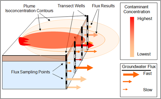
Figure 1-19. Measuring mass flux using wells along a transect. Results illustrate spatial variations in mass flux across a contaminant plume.
Source: (Graphic courtesy HydroGeoLogic Inc.) Figure 2-4. in ITRC Use and Measurement of Mass Flux and Mass Discharge (ITRC 2010).
1.3.8.3 Selection of Analytical Methods
There has been rapid development of a variety of methods for analyzing environmental media for PFAS and other fluorinated compounds. When selecting methods, their utility and limitations should be understood to avoid employing unnecessary methods or inaccurate interpretation of results. See Section 11.2 for more information about analytical methods.
The following list provides suggestions and caveats for strategic use of these methods:
- Target analyses—Target analytical methods (for example, USEPA Method 1633A, USEPA 2024) are most commonly used and appropriate for PFAS site investigations. They use certified calibration standards to detect and quantify a list of specific PFAS in a variety of environmental media. Often, the full method analyte list is run, particularly for initial site investigation. Multiple analytes allow for: 1) forensic assessment, 2) determination of firefighting foam composition, 3) identification of precursors and associated transformation, 4) PFAS fractionation evaluation, and 5) accounting for type and mass of multiple PFAS affecting treatment and remediation. Reducing the reporting list may be warranted after collection of a robust data set and thorough investigation of potential PFAS sources.
- Non-targeted analyses — Combined with a suspect screening search, non-targeted analyses can identify the presence of a broad range of PFAS not typically reported with target analytical methods. Non-targeted analyses, such as quadrupole time-of-flight (qTOF), are useful for forensic purposes and to validate the detection of individual PFAS by target analyses but are not quantitative. Non-targeted analysis may also identify unexpected PFAS that may warrant additional inquiry or explanation. See Section 11.4.3.
- Total organic fluorine analyses—Analytical methods for the detection of total organic fluorine, such as adsorbable organic fluorine or extractable organic fluorine, have been in recent development. Results may include PFAS and non-PFAS and do not identify individual PFAS or other compounds. These methods typically have higher method detection limits than target analyses. Of these methods, USEPA Method 1621, Determination of Adsorbable Organic Fluorine in Aqueous Matrices by Combustion Ion Chromatography, is multilab-evaluated and accredited for compliance monitoring (USEPA 2024; see Section 11.2.2.4). This type of analysis may be useful for applications such as treatment system design or performance monitoring by mass removal, where the system is affected by all organofluorine molecules. This type of analysis should not be used as a site investigation “dragnet” for the broad detection and identification of PFAS. Such an approach would result in nonspecific results that could be affected by non-PFAS or unregulated PFAS with no criteria for evaluation, potentially creating an unfounded inference that the site is adversely affected by regulated PFAS.
- TOP assay—This method has been in existence for several years and is generally well established. The method subjects a sample to aggressive oxidation conditions, which forcibly transforms precursor PFAS to fully fluorinated terminal PFAS. It is useful to evaluate the potential for precursor transformation in the environment or within certain treatment systems (for example, emerging destructive technologies such as supercritical water oxidation [SCWO]). It can also be used to normalize concentrations of samples in various stages of precursor degradation for forensic comparison. Ateia et al. (2023) provided additional insight for the applications and challenges of TOP assay. The oxidation step in TOP assay transforms precursor PFAS to terminal PFAAs, but the terminal products in this reaction are not necessarily the same as the ones that would be produced in nature. For example, TOP assay transforms PFSA precursors into PFCAs. Also, the strongly oxidizing conditions can result in chain-cutting reactions, such that the mixture of PFAA compounds produced may be smaller on average than would be found under normal environmental conditions. TOP assay results should not be construed to indicate that precursors will necessarily degrade to terminal degradation products in the environment because TOP assay laboratory conditions do not represent field conditions (see Section 11.2.2.2 for more information about the TOP assay).
1.3.8.4 Appropriate Application of Criteria
Regulatory criteria have been (and are being) developed for PFAS in a variety of environmental media with certain ecological and human exposure scenarios in multiple jurisdictions (see the Environmental Media Values Table). Sometimes these criteria are misapplied out of a sense of caution/conservatism, convenience, or due to misunderstanding of the CSM. Certain comparisons may be protective as a screening-level evaluation but may warrant additional site-specific assessment before they drive remedial action. Examples include comparing leachate concentrations to groundwater criteria or comparing groundwater results to surface water criteria. Investigation data should be collected in a manner that supports comparison to applicable regulatory criteria.
- Drinking water criteria are not necessarily applicable to groundwater concentrations. Drinking water criteria are commonly the basis for groundwater remediation standards. In some instances, groundwater may be nonpotable, restricted, or of insufficient yield. Turbid groundwater samples can reflect an elevated PFAS concentration in water that would not be consumed by humans due to the turbidity. Well development/rehabilitation and proper well construction should be implemented to reduce turbidity for groundwater samples that are more representative of potential drinking water. In some instances, groundwater criteria are based on various aquifer classifications or use scenarios. Criteria should be selected according to site conditions and setting. Exceeding a generic drinking water criterion may warrant further evaluation.
- Soil leachate sample results do not represent groundwater concentrations. PFAS in soil leachate samples (for example, synthetic precipitation leaching procedure [SPLP]) are measured under laboratory conditions and differ from field leachate concentrations (see Section 1.3.8.6 for additional information about leaching). Leachate may undergo additional processes before encountering groundwater (for example, resorption as leachate migrates through the vadose zone, precursor transformation, and dilution in groundwater). Leachate sample results should be compared to leachate-specific regulatory criteria where these criteria exist. Otherwise, a site-specific evaluation relative to potential groundwater impacts may be warranted (see Section 1.5.1).
- Groundwater results do not represent surface water concentrations. Groundwater discharge to surface water often involves additional sorption to organic sediments, enhanced sequestration to sediments due to brackish or saline porewater, and dilution in the surface water body. If groundwater concentrations exceed surface water criteria, additional evaluation is warranted. Refer to Section 1.3.4 on PFAS Groundwater-Surface Water Interactions and Section 1.3.8.2 on Surface Water Receptors for a mass-flux approach to evaluate the potential impact to surface water.
- There are multiple factors for surface water criteria. Surface water criteria are commonly very stringent (close to analytical detection limits) due to the potential for bioaccumulation of PFAS to higher trophic levels, other ecological effects, and for protection as drinking water. Ecological criteria for surface water may be less stringent when they reflect the effect of PFAS on certain organisms without bioaccumulation. In some instances, there are surface water criteria for human recreation, based on dermal exposure and limited/incidental ingestion; these tend to be less stringent. Surface water criteria may also be differentiated based on fresh versus brackish versus seawater; these should not be used interchangeably. Emerging human health concerns, unrelated to drinking water, are also driving stringent criteria (for example, full-body-contact recreation sites, aquatic life harvesting, and subsistence fishing).
1.3.8.5 Repurposing and Refining the Conceptual Site Model
PFAS may occur at a site for which a CSM has already been developed for other contaminants. In this case, it can be efficient and cost-effective to use findings and elements from the existing CSM for purposes of the PFAS investigation. Such elements include hydrostratigraphic framework, groundwater flow direction, seepage velocity, aquifer structural/matrix properties, pathways, and receptors. In some instances, PFAS may interact with other known contaminants (for example, NAPL) that should be accounted for in the CSM. In most cases, the CSM will likely require additional PFAS-specific spatial, physical, and chemical information to be useful and reliable.
Characterization of PFAS vertically through the soil profile is an important aspect of the PFAS CSM, due to unique retention properties (for example, air-water interfacial sorption) and accumulation at discrete horizons (for example, clay– or organic carbon–enriched layers). Pre-existing, detailed soil characterization can be repurposed in the PFAS CSM or profiled in detail for the first time to support the PFAS CSM. Continuous and discrete vertical characterization of PFAS in the soil profile should be considered (at least at targeted locations) and can be augmented with potentially unconventional tools such as lysimeters to characterize PFAS concentration in porewater/retained at the AWI.
A strategic consideration for the PFAS CSM is the effect of the capillary fringe (tension-saturated zone above the water table and below the unsaturated zone). Fluctuations in the capillary fringe may mobilize PFAS (Das et al. 2024), especially where they are otherwise retained by air-water interfacial sorption. Porewater characterization (for example, sampled with lysimeters) of the capillary fringe is a means to quantify aqueous concentrations of PFAS in this zone of saturation above the water table, which could not otherwise be sampled via a monitoring well.
PFAS CSMs should also account for migration, attenuation, and transformational processes affecting PFAS: precursor degradation, sorption, dispersion, and matrix diffusion (Kornuc et al. 2022; Newell et al. 2021; Newell et al. 2021). Adamson et al. (2022) noted the marked concentration reduction of PFAS measured in groundwater along the migration pathway from the source areas, attributing this to nondestructive retardation/retention processes of hydrophobic, air-water interfacial sorption, and electrostatic partitioning. Section 5 includes information about PFAS fate and transport process.
1.3.8.6 PFAS Characterization by Media and Pathway
This section describes the approach, tools, and techniques for sampling and investigation design. Figure 1-20 presents a conceptual graphic for the characterization of PFAS, using an AFFF site as an example. Sites with other PFAS sources may require different conceptualization for investigation design.
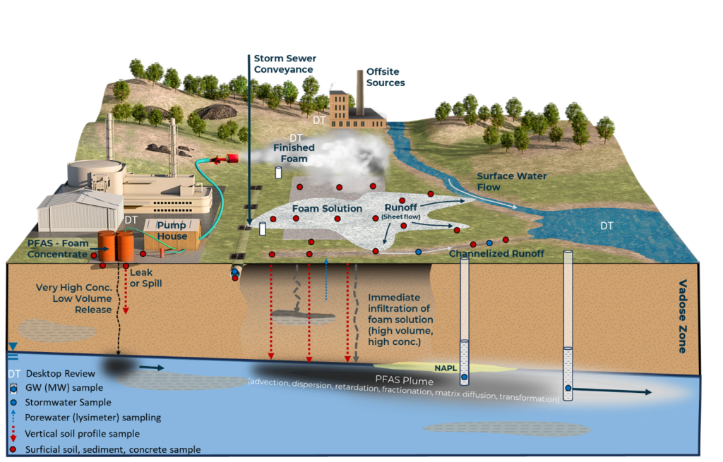
Figure 1-20. Illustrated PFAS characterization approach.
Source: J. Hale and J. West, Kleinfelder. Used with permission.
Beyond sampling for PFAS specifically, several site-specific parameters related to soil and aquifer matrix properties and solutions chemistry affect the partitioning, mobility, and distribution of PFAS. These include soil type (mineralogy and grain size), pH, and organic matter/total organic carbon (TOC) (Hubert et al. 2023; Feng et al. 2024; Wanzek et al. 2023). Refer to Section 5.2 for information about phase partitioning. For information about collecting samples for PFAS, refer to Section 11.1.
Soil
Many PFAS (for example, PFOS) are sorptive, recalcitrant, and nonvolatile. When released to the surface of soil, they may be retained for relatively long durations (depending on soil characteristics), preserving the pattern of the original surface release. High-density, shallow soil sampling of suspected source areas and drainage ways for PFAS analysis is often appropriate. This can be conducted by manual methods (for example, hand-auger, shovel, or trowel) or direct-push sampling apparatus. Designating a percentage of these samples (spatially distributed) for PFAS leachate analysis (for example, SPLP) will provide an indication of PFAS leaching potential. As noted above, laboratory leachate results are not a direct indicator of expected groundwater PFAS concentrations. Consider also sampling soil downwind (which may be hydraulically upgradient) where PFAS may have migrated by aerial dispersion and deposition or deposition by mist drift, as with firefighting foam.
Though retained in shallow soil, PFAS are commonly distributed vertically through the vadose zone, partitioning to organic carbon and charged mineral surfaces (Figure 1-21). PFAAs and other amphiphilic PFAS are also retained by air-water interfacial adsorption, which is unique to this class of contaminants (Brusseau et al. 2019; Brusseau and Van Glubt 2019). See Section 1.3.1 for more information about vadose zone characterization and transport and Section 1.5.1 for information about leaching methods. Retention by air-water interfacial sorption is transient and cyclic, as PFAS may be leached and mobilized to groundwater by infiltration and subsequently resorbed, as air and water phases return in the pore space. Inversely, PFAS may also be mobilized vertically upward in the soil profile because of evapotranspiration or fluctuation of the capillary fringe (Wallis et al. 2022). Figure 1-21 illustrates a hypothetical example vertical PFAS concentration profile relative to soil type and TOC concentration. The figure shows the discrete vertical distribution of PFAS both by concentration and proportion of individual PFAS and how they are affected by discrete soil characteristics.
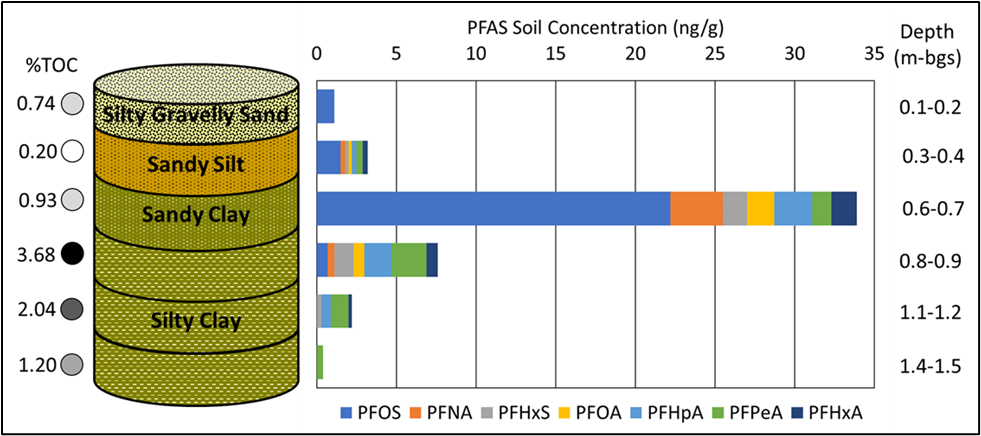
Figure 1-21. Hypothetical example of PFAS vadose zone distribution and matrix. Depth given in meters below ground surface (m-bgs).
Source: J. Hale, Kleinfelder. Used with permission.
Table 1-7 provides a summary of the types of soil characteristics that can be collected to produce a vertical profile of the vadose zone, including the purpose or utility and suggested sampling frequency for each category of soil characteristics. Campos-Pereira et al. (2023) described the effects of pH, surface charge, and soil properties on PFAS partitioning to solids in a variety of soils. A proportion of surface soil sample locations should be designated for vertical profiling, selected to provide spatial coverage, and biased toward areas of natural runoff. High-resolution and depth-discrete soil sampling is consistent with the approach taken by Kornuc et al. (2022).
Table 1-7. Vertical soil profile sampling
| Testing/Analysis | Purpose | Sample Selection |
|---|---|---|
| Field Description | ||
| Texture, Grain Size, Moisture | Understanding of soil type; cofactors in PFAS sorption & leachability | Continuous vertical description |
| Soil Mineralogy | ||
| Color | ||
| Organic Matter, Staining, NAPL | ||
| PFAS | ||
| Soil PFAS | PFAS distribution in soil profile | One sample per discrete interval (0.5 ft or 0.1 m) |
| SPLP PFAS | Leachability of PFAS and correlation to soil concentration | |
| Porewater PFAS | PFAS porewater concentrations and migration to groundwater potential | Collected via dedicated lysimeters over time to capture range of infiltration and soil moisture conditions |
| Geotechnical, General Chemistry, & Matrix Parameters | ||
| Grain Size (sieve and hydrometer) | Understanding of soil type; cofactors in PFAS sorption & leachability | One sample per soil type per boring |
| Unified Soil Classification System (USCS) Soil Classification; Engineering | ||
| Soil Mineralogy | ||
| Soil pH | ||
| Soil Salinity/Conductivity | ||
| Anions (sulfate, fluoride, chloride) |
One sample per soil type (minimum one sample from each material type comprising the soil; samples from multiple locations preferred) |
|
| Cations (Ca2+, Mn2+, Mg2+, Fe3+) | ||
| Cation/Anion Exchange Capacity | ||
| Moisture Content | One sample per discrete interval (0.5 ft or 0.1 m) | |
| Total Organic Carbon (TOC) | ||
Table 4-1 shows that laboratory and field studies have resulted in a wide range of sorption values (Kd or Koc) for individual PFAS, indicating the degree of sorption or leaching for various PFAS species is highly dependent on the setting due to parameters noted above. Because of this variation, some regulatory agencies, including the USEPA, advise the derivation and use of site-specific sorption coefficients to inform potential risk of PFAS leaching to groundwater. Two common methods are discussed in USEPA (2025) and are summarized below. Navarro et al. (2024) provided a comprehensive summary of additional methods for evaluating PFAS leaching from soil and other solid materials.
SW-846 Test Method 1312: Synthetic Precipitation Leaching Procedure is a relatively common method for assessing PFAS leachability from soil (USEPA 1994). The procedure involves mixing an extraction fluid composed of reagent water adjusted to a pH of 4.2 or 5.0 (depending on the sample’s geographical origin) with a mix of nitric and sulfuric acids and shaking the mixture for 18 hours with the intent to simulate natural leaching in the environment. The USEPA (2025) guidance described a modified SPLP procedure that is specific to PFAS. Modifications include differences in materials as well as a reduction of sample volume and the use of a methanol solution for total extraction in parallel with the standard extraction fluid.
Lysimeters can be used to extract and analyze porewater from the vadose zone and capillary fringe, where PFAS may be sequestered via air-water interfacial sorption. Lysimeters are purged by applying vacuum to the system, which moves porewater through the apparatus into a secondary containment vessel. The sample volume from each purge event of the lysimeter may be less than the required volume for analysis. In this case, samples from multiple events may need to be composited or arrangements made with the laboratory to analyze a lesser sample volume. Ideally, samples will be acquired during discrete events that reflect the then-current porewater saturation and infiltration conditions. USEPA (2025) noted that while lysimeters have the advantage of measuring actual pore water conditions at a site, there are uncertainties regarding whether commonly used materials in lysimeters adsorb PFAS and the implementation and interpretation of results is complex compared to SPLP. Results of studies using lysimeters to derive site-specific values to protect groundwater should be interpreted with caution.
Groundwater
In some circumstances, existing monitoring wells are useful for initial groundwater characterization of PFAS. The following considerations should be evaluated when using an existing monitoring well network for initial PFAS investigation:
- location of monitoring wells relative to the suspected source and in the downgradient direction, informed by PFAS soil characterization results
- depth and screened interval of monitoring wells
- status of monitoring well construction, development, and rehabilitation
- potential for prior use of PFAS-containing materials in the construction of the monitoring wells
- presence of NAPL
Notably, turbidity in monitoring wells is problematic due to the sorptive nature of certain PFAS and the low detection/regulatory criteria (ng/L) for PFAS. Consequently, redevelopment of existing monitoring wells, and proper design (screen slot size and filter pack) and development (bidirectional surging, purging, and field parameter monitoring) of new monitoring wells, are important to reduce turbidity. The analytical laboratory should be consulted if the groundwater samples remain visually turbid.
In the absence of suitable existing monitoring wells, new monitoring wells should be installed based on knowledge of PFAS sources and groundwater flow directions, informed by the desktop review and surficial soil sampling. Monitoring wells should be constructed with and installed using PFAS-free equipment and materials. As an example, the US Navy conducted a study on coated bentonite pellets used in monitoring wells and found PFAS in the leachate from several different brands of pellets (Radford et al. 2023). Drill cuttings and purge water may have special handling and disposal requirements based on the potential presence of PFAS.
PFAS are soluble, so screen interval and placement should not be based on expectations of a “floating” or “sinking” separate phase, but rather potential for vertical hydraulic gradients. The occurrence of PFAS in groundwater will be determined during the initial phase of PFAS characterization sampling of groundwater monitoring wells. Similar to other solutes, PFAS in groundwater migrate by advection and dispersion and, depending on the specific PFAS, may be subject to varying degrees of retardation (though generally expected to be less than in the vadose zone). Investigators should obtain hydraulic conductivity from existing site characterization information or conduct aquifer testing (for example, slug or pumping tests) by conventional means for the calculation of seepage velocity, if needed. Aquifer matrix characteristics and aquifer chemistry influence the sorption of and potential precursor transformation of PFAS. Refer to Table 1-8 for aquifer matrix and groundwater chemistry parameters for measurement and analysis.
Table 1-8. Aquifer matrix and groundwater chemistry sampling
| Testing/Analysis | Purpose | Sample Selection |
|---|---|---|
| Field Parameter Measurements | ||
| pH | Lower pH (elevated hydrogen ion activity [H+]) enhances anionic PFAS sorption (reduced aqueous concentration) | Measure with field meter at every monitoring well sampled |
| Salinity/Specific Conductivity | Positively correlated to PFAS sorption (reduced aqueous concentration) | |
| Oxidation-Reduction Potential (ORP) | Oxidizing conditions conducive to aerobic precursor transformation; reducing conditions limit aerobic transformation | |
| Turbidity | PFAS adhere to solid particles and colloids. Turbidity can affect and skew PFAS concentration results | |
| Aqueous Laboratory Analyses | ||
| Calcium Ion (Ca2+) Concentration | Positively correlated to PFAS sorption (reduced aqueous concentration) | Discretionary analysis for more robust characterization of sorption influences |
| Aquifer Matrix Parameters | ||
| Grain Size (sieve and hydrometer) | Understanding of aquifer matrix and permeability | Laboratory analysis. Obtain from prior investigation or collect from saturated zone when installing monitoring wells for PFAS sampling (minimum one sample from each material type composing the aquifer matrix; samples from multiple locations preferred) |
| USCS Soil Classification; Engineering | ||
| Total Organic Carbon (TOC) | Positively correlated to PFAS sorption (reduced aqueous concentration) | |
| Cation/Anion Exchange Capacity | Cofactors in PFAS sorption & leachability | |
| Bulk Density | Fate & transport retardation parameter | |
| Effective Porosity | Key parameter for seepage velocity of dissolved PFAS | Select samples of aquifer matrix (in saturated zone) acquired via borings or in conjunction with monitoring well installation |
| Aquifer Hydraulic Characteristics | ||
| Hydraulic Conductivity | Key parameter for seepage velocity of dissolved PFAS | Slug testing of select monitoring wells or aquifer testing. Data may exist from prior site characterization |
Retention of PFAS in Concrete
PFAS are known to partition into and leach from concrete. Consequently, concrete surfaces (for example, fire training pads, storm sewers) represent sinks and sources of PFAS. PFAS in concrete can be characterized by coring, cutting into discrete disks, and laboratory analysis of PFAS and PFAS in leachate (for example, SPLP). Alternatively, PFAS-free water can be rinsed over or maintained in contact with concrete surfaces and subsequently analyzed for the accumulation of PFAS in the water. The phenomena of PFAS sorption and release from concrete, along with methods for analysis, are addressed by Thai et al. (2025, 2025). See Section 1.5.6 for more information about concrete and asphalt sampling and analysis.
Surface Water Runoff and Storm Sewer Flow
Informed by the desktop analysis, investigators should sample soil and sediment from stormwater conveyances and accumulation features (swales, drainage channels, and stormwater sewer pipes) that may convey PFAS from the source or release locations.
Even after PFAS have partitioned into environmental media following release or application, conveyance by stormwater flow may occur. PFAS can be desorbed from soil, sediment, and concrete during transient precipitation events, or soil and sediment with sorbed PFAS may be mobilized by stormwater flow. Collect aqueous samples of stormwater runoff and storm sewer flow based on prior soil/sediment sampling and desktop review. It may be necessary to coordinate this sampling with forecasted precipitation or simulate the flow, as with concrete washing.
–
Updated January 2026.

